Quickly format a range of cells by choosing a table style. You can also create your own table style. Quickly format a cell by choosing a cell style.

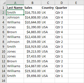
1. Click any single cell inside the data set.

2. On the Home tab, in the Styles group, click Format as Table.

3. Choose a table style.

Note: click New Table Style to create your own table style or right click a table style and click Duplicate to create a new table style that is similar to an existing one. Modifying a custom table style affects all tables in a workbook that use that table style. This can save a lot of time.

4. Excel automatically selects the data for you. Check ‘My table has headers’ and click on OK.

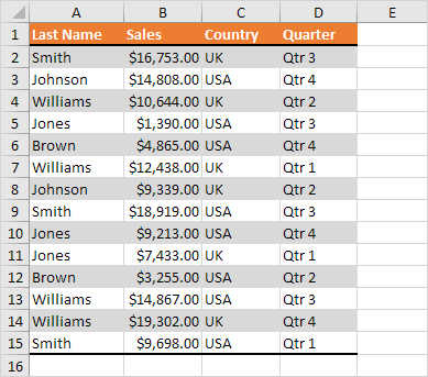
Result. This is another way to insert a table.

To convert this table back to a normal range of cells (and keep the formatting), execute the following steps.

5. First, select a cell inside the table. Next, on the Design tab, in the Tools group, click Convert to Range.

Result. A nicely formatted range of cells.

Note: to remove the table style, select the range of cells, on the Home tab, in the Styles group, click Normal.