Excel SUBSTITUTE Function
Replacing a text with some other text is a common job that we all do in Excel, and we all have different ways to do so. But do you know that Excel has provided an inbuilt function named SUBSTITUTE to replace one or more instances of text strings with another. In this tutorial, we will take a deeper look at the SUBSTITUTE function.
What is SUBSTITUE function?
The Excel Substitute function replaces a part of the text in a string with some other text. SUBSTITUTE function is used to clean data by substituting one or more characters from imported data. For example, if we have imported some data from a PDF file in a format 458-299-605, we apply the SUBSTITUTE function to transform it into 458299605.
The Excel SUBSTITUTE function replaces or substitutes the text strings with other text strings. You can use the SUBSTITUTE function to replace the text based on matching (remember, it doesn’t work with position). You can also replace one or more text strings with no data; you need to pass an empty string (“”) in the argument. SUBSTITUTE is an inbuilt function categorized under Excel Text Functions.
SUBSTITUTE function is case-sensitive. You can use it as a worksheet function in Excel. The SUBSTITUTE function can be inserted as part of another formula in a cell as a worksheet function. This function allows you to substitute the text in strings easily, and it gives you the ability to decide which part of the string you want to replace. The alternative option of this function is to use the Find and Replace Excel feature.
NOTE: A single SUBSTITUTE function can only replace one text value at a time. However, you can nest the SUBSTITUTE function inside of itself to replace more than one string.
Syntax
Parameters
- Text (Required): This argument specifies the text in which you want to substitute the text.
- Old_Text (Required): This argument specifies the old text which you want to replace.
- New_Text (Required): This argument specifies the new text with which you want to replace your original text.
- Instance_number (optional): The occurrence of old text which you want to replace with new text. When you skip the instance parameter, all occurrences of the old_text argument are replaced with the new_text argument.
Points to Remember for SUBSTITUTE function
- SUBSTITUTE function searches and replaces the old_text argument with new_text in a specified string.
- Instance limits SUBSTITUTE replacement a particular instance of old_text.
- When you skip the instance parameter, all occurrences of the old_text argument are replaced with the new_text argument.
- The SUBSTITUTE is a case-sensitive function and it does not support wildcards.
Example 1: Use SUBSTITUTE function to make changes to some of the strings below to get the results mentioned in the ‘Result’ column.
| String | Instances | Result |
|---|---|---|
| Bob | Bot | |
| Bumble | 1 | Tumble |
| Excel is easy to use | Excel is convenient | |
| The Excel is the easy application | 2 | The Excel is an easy application |
| The Excel is the popular application | Excel is the popular language |
To SUBSTITUTE you data follow the below given steps:
STEP 1: Add a helper column named Output
Place your mouse cursor to the cell next to “Result” and name the new column as “Output”.
It will look similar to the below image:

We will type our SUBSTITUTE formula in this column and place the SUBSTITUTE data for different text values.
NOTE: Format the helper column and match it with the match column to make your Excel sheet more attractive.
STEP 2: Type the SUBSTITUTE formula
Put your cursor to the second row and start typing the function: = SUBSTITUTE(
It will look similar to the below image:

STEP 3: Insert the parameters
- Text: Here we will specify the text that we want to change. It is the reference cell of the string, i.e. B4 OR HUT, so our formula becomes: =SUBSTITUTE(B4,

- Old_text:In this parameter, we will specify the string (of our existing text string) we want to change. Here, in our case, we want to change the string b, so type it in with double quotations, i.e. “b”, so our formula becomes: =SUBSTITUTE(B4, “b”,

- New_text:In this, we will specify the change we want to Old_text. It will be entered in double quotations. Unlike here, we want to substitute Old_text with “t”, so our formula becomes =SUBSTITUTE(B4, “b”,”t”

- Instance_num:This parameter indicates which specific instance we are targeting the substitution on. Since here there is only one occurrence of “b” so we will skip this optional parameter.
Our final formula will look similar to the below image: 
STEP 4: SUBSTITUTE will return the result
The SUBSTITUTE will replace the character “b” with “t” and will return the output as “Bot”.
It will look similar to the below image:

STEP 5: Repeat the formula for the other rows
- In the E5 cell, type the formula: = SUBSTITUTE (B5,”B”,”T”,1). Since Bumble has two b’s, we have specified in instance 1, so it will substitute the first instance of b with alphabet T.

- In the E6 cell, type the formula: =SUBSTITUTE (B6,”easy to use”,” convenient”). This function will replace the string “easy to use” with convenient as shown in the below image:

- In the E7 cell, type the formula: =SUBSTITUTE (B7,”the”,”an”,2). Since the text “the Excel is the easy application” has two the’s. Therefore we have specified in instance 2, so it will substitute the second instance of ‘the’ with the alphabet “an”.

- In the E8 cell, type the formula: =SUBSTITUTE (B8,”The”,” “). The SUBSTITUTE function is case-sensitive. Therefore it will treat “The” and “the” as different strings. This function will replace the string “The” with an empty string.

Refer to the below image for all the outputs:

That’s it, and now you have successfully learnt how to use the SUBSTITUTE function in Excel. Let’s explore some complicated examples.
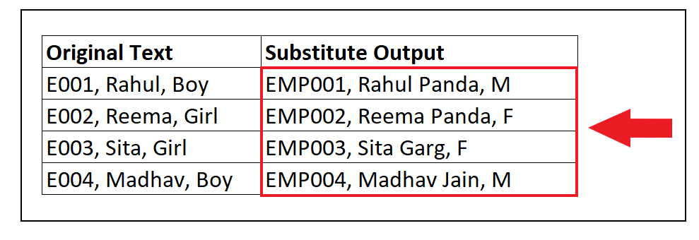
Example 2: Demonstrate the use of nested SUBSTITUTE function using below table:
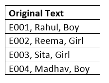
The SUBSTITUTE function cannot replace more than one string in a single function. Since in the above table, we have to replace all the three strings, we need to have three separate SUBSTITUTE functions in the same cell and get three of them replaced. To achieve this, the best method is to nest ONE SUBSTITUTE function inside other.
To understand nested SUBSTITUTE functions follow the below-given steps:
STEP 1: Add a helper column named SUBSTITUTE Output
Place your mouse cursor to the cell next to “Original Text” and name the new column as “SUBSTITUTE Output”.
It will look similar to the below image:
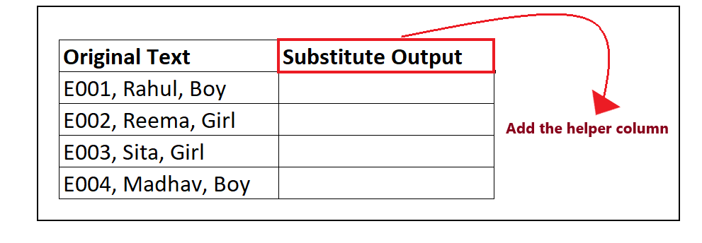
We will type our SUBSTITUTE formula in this column and place the SUBSTITUTE data for different text values.
STEP 2: Type the SUBSTITUTE formula
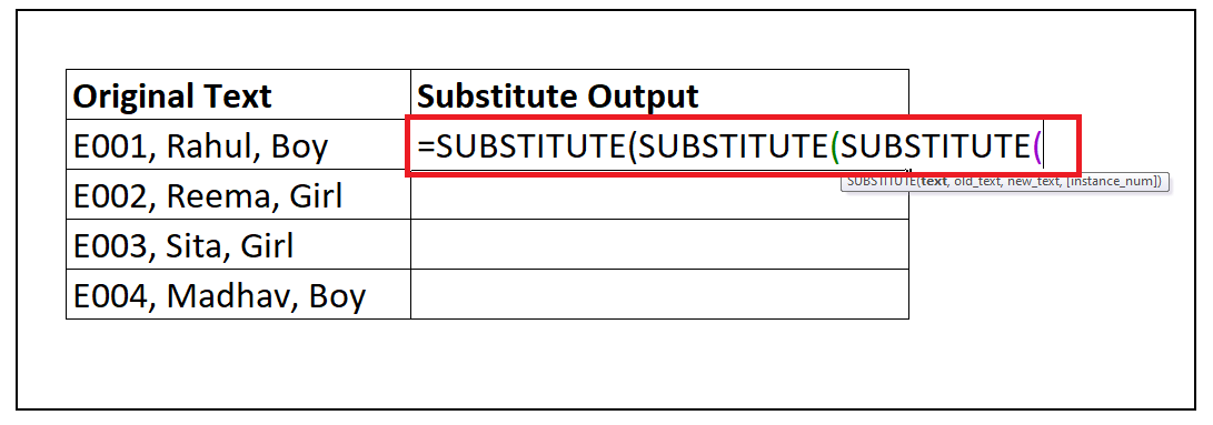
- Put your cursor to the second row and start the nested formula by typing: = SUBSTITUTE(
- Since have three strings that we want to replace therefore we will nest three SUBSTITUTE functions one inside another. The formula will be: =SUBSTITUTE(SUBSTITUTE(SUBSTITUTE(
STEP 3: Insert the parameters of the nested substitutes
- Firstly we will enter the parameter for the third SUBSTITUTE function. We will replace the string “Boy” with string “M”. The formula will become: =SUBSTITUTE(SUBSTITUTE(SUBSTITUTE(C4,”Boy”,”M”)

- Next, we will enter the parameters for the second SUBSTITUTE function. We will replace the old string “Rahul” with the new string “Rahul Panda”. In the second nested function, you don’t require to put the text parameter again; we will only specify the Old_Text and New_Text arguments. The formula will become: =SUBSTITUTE(SUBSTITUTE(SUBSTITUTE(C4,”Boy”,”M”),”Rahul”,”Rahul Panda”),

- For the third nested function, add the parameters. We will replace the old string “E001” with the new string “EMP001”. In the third nested function, you don’t need to put the text parameter again; we will only specify the Old_Text and New_Text arguments. The formula will become:
=SUBSTITUTE(SUBSTITUTE(SUBSTITUTE(C4,”Boy”,”M”),”Rahul”,”Rahul Panda”),”E001″,”EMP001″)
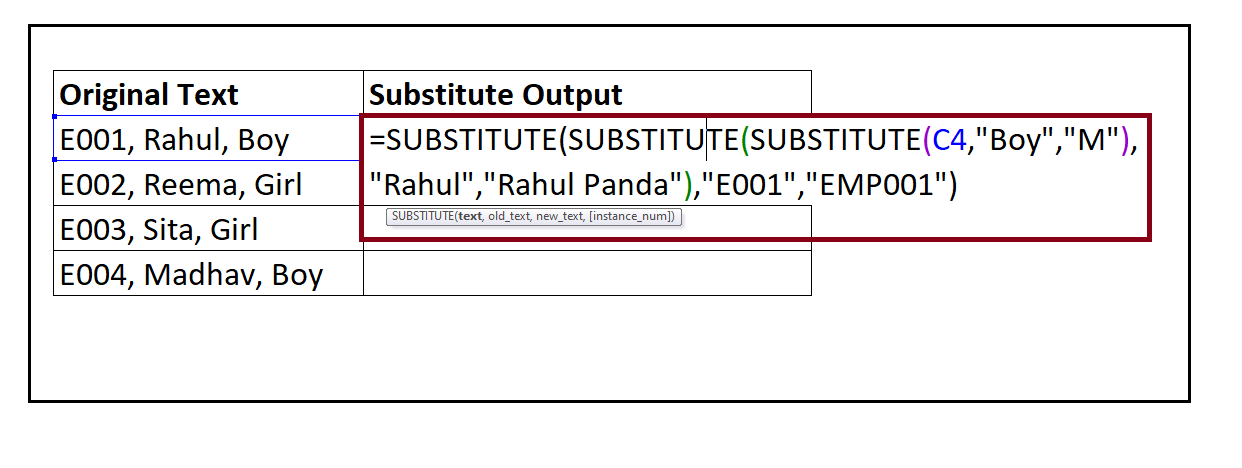
Our formula will look similar to the below image:
STEP 4: SUBSTITUTE will return the result
The nested SUBSTITUTE functions will replace all the old strings with the new strings and will return the data at once.
The output will look similar to the below image:

STEP 5: Repeat the above formula for the following rows
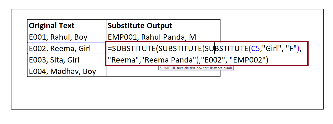
- In the D5 cell, type the formula: =SUBSTITUTE(SUBSTITUTE(SUBSTITUTE(C5,”Girl”, “F”),”Reema”,”Reema Panda”),”E002″, “EMP002”).
It will replace all the Old_Text with the New_Text and give you the result.
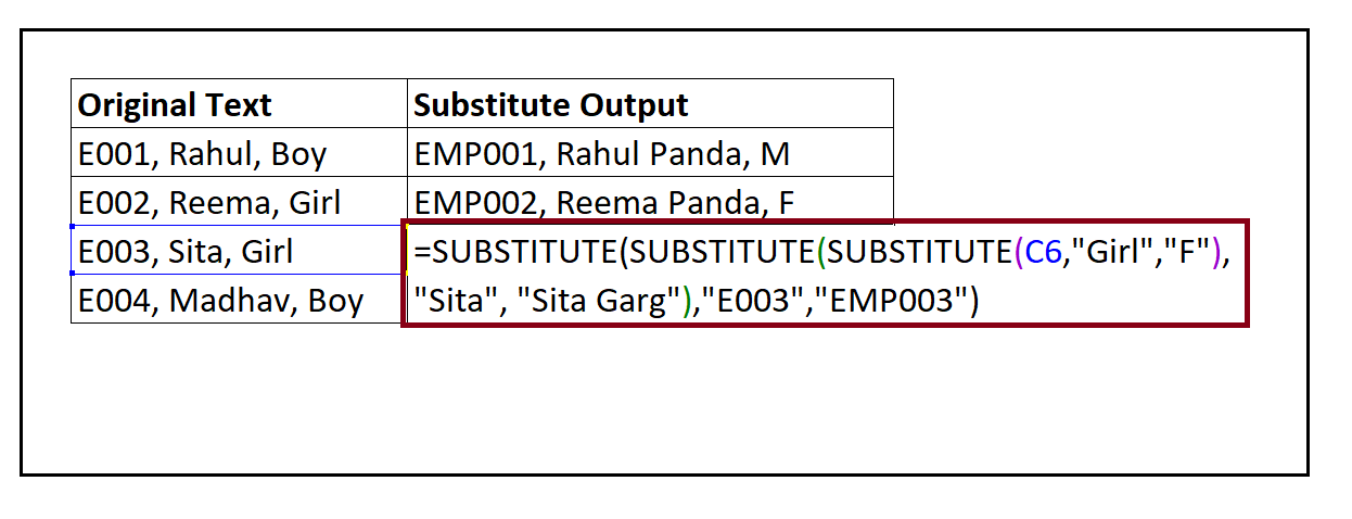
- In the D6 cell, type the formula: =SUBSTITUTE(SUBSTITUTE(SUBSTITUTE(C6,”Girl”, “F”),”Sita”, “Sita Garg”),”E003″,”EMP003″)
- In the D7 cell, type the formula: =SUBSTITUTE(SUBSTITUTE(SUBSTITUTE(C7,”Boy”,”M”),”Madhav”,”Madhav Jain”),”E004″,”EMP004″).
It will replace all the Old_Text with the New_Text and give you the result.
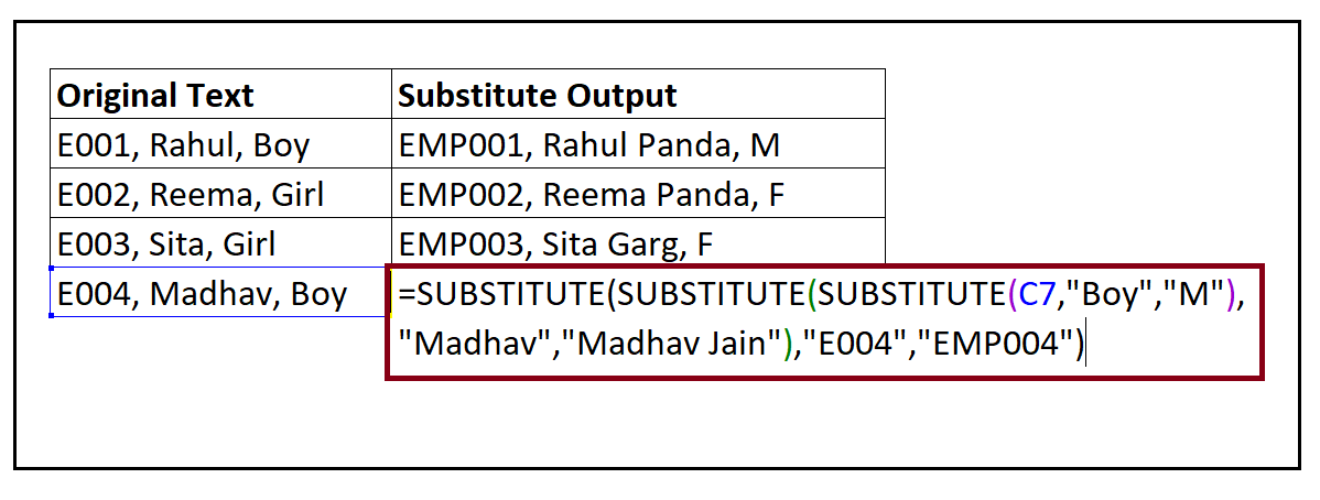
The nested SUBSTITUTE functions will replace all the old strings with the new strings and will return the output for all the rows.
Refer to the below image:
Example 3: Using the SUBTITUTE function remove the line breaks from your Excel worksheet.
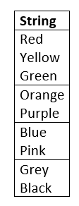
To replace the line breaks from the text, you can use a combination of SUBSTITUTE and CHAR functions. To remove the line breaks from your cells follow the below-given steps:
STEP 1: Add a helper column named SUBSTITUTE Output
Place your mouse cursor to the cell next to “String” and name the new column as “Output”.
It will look similar to the below image:
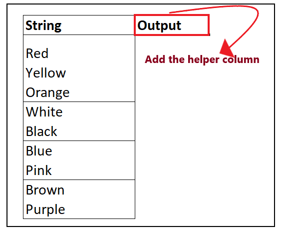
In this column we will type our SUBSTITUTE formula and place the SUBSTITUTE data for different text values.
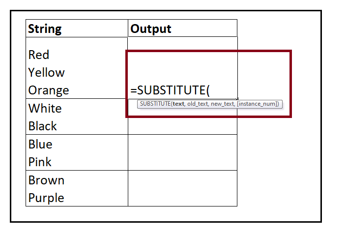
STEP 2: Type the SUBSTITUTE formula
Put your cursor to the second row and start typing the function = SUBSTITUTE(
It will look similar to the below image:
STEP 3: Insert the parameters
SUBSTITUTE can locate matching text anywhere in a cell and replace it with the text of your choice. SUBSTITUTE can accept up to four arguments, but we will use only the first three and skip the fourth parameter.
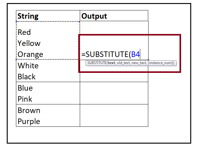
- In the text parameter, we will specify the string from which we want to remove the line breaks. It is the reference cell of the string, i.e. B2, so our formula becomes: =SUBSTITUTE(B4,
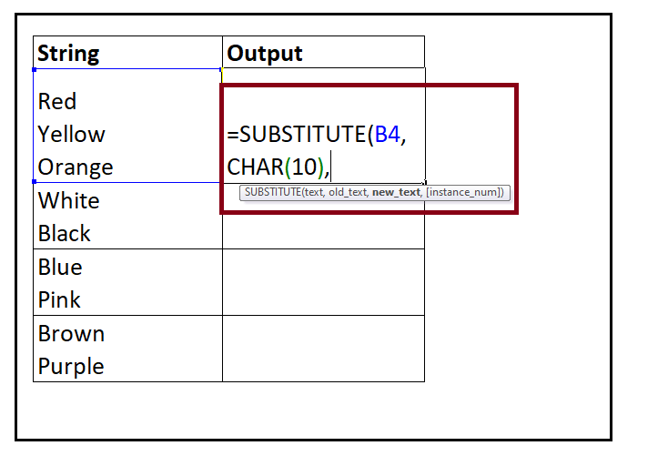
- In the second parameter (Old_text) we will specify the line break as that is what we want to substitute. We know that the ASCII character set is CHAR(10) in excel, so our formula becomes: =SUBSTITUTE(B2, CHAR (10)
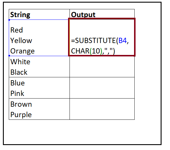
- In the third parameter we will specify the new text with which we want to replace the old text which in our case is comma (,), so our formula becomes: =SUBSTITUTE(B5,CHAR(10, “,”)),”, “)
Refer to the below image:
STEP 4: SUBSTITUTE will return the result
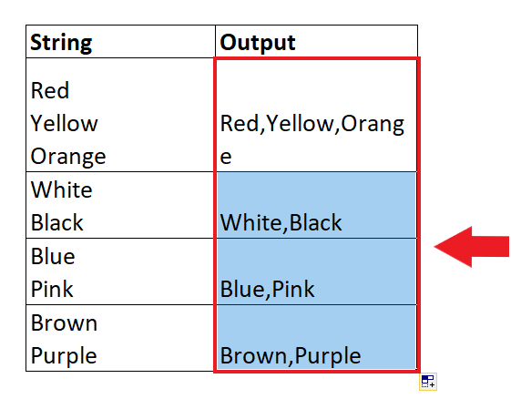
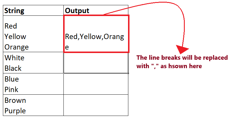
The SUBSTITUTE function will replace all line breaks or Char (10) characters with comma (,) from B4 cell and will return the final output i.e, “Red, Yellow, Orange” in cell C4.
Refer to the below image:
STEP 5: Drag the formula to other rows to repeat
- Place your mouse cursor on the formula cell and point the cursor to the right corner of the cell. To your surprise, the mouse pointer will turn into a ‘+’ icon.
- Drag the ‘+’ icon down the cells. It will copy the SUBSTITUE function to all your cells changing the cell reference as respective to the cell.
