How to add page break in Excel?
An Excel sheet can be divided into multiple pages/parts prior to printing. The user can break an Excel spreadsheet into several parts by using the page break feature of Excel. A page break is a line divider used in an Excel spreadsheet to separate the data into different sections.
Note: Page break can be inserted vertically and horizontally.
Excel automatically handles pages breaks, but sometimes you need to manage the page break manually to insert it as the way you want in a vertical page break.
This chapter will describe each step to insert a page break to an Excel worksheet using two different methods. Each method is equally important. You can use any of them which you find easy and simple.
What is a page break? How is it used?
Page break is commonly used in an Excel spreadsheet, when you want to separate an Excel sheet data into different sections or a single Excel sheet consisting of several tables data. Page breaks give control to the users if they don’t want that a row to be printed on a page.
To separate these data, page breaks are used so that it becomes clear for reading and understanding.
A page break is a line divider that marks the edges of each page. You can insert the page break vertical and horizontal as well. The Excel page break helps the users to analysis that where page break will appear while printing the Excel worksheet.
Properties of page break
- You can add any number of page breaks to an Excel sheet.
- Excel allows to insert the vertical and horizontal page breaks to an Excel sheet.
- All page breaks added to an Excel sheet can be removed at once and one-by-one also.
Types of page breaks
Excel offers two types of page breaks:
- Solid line page break (Manually added)
- Dashed line page break (Automatically added)
Solid line page breaks are manually added to an Excel spreadsheet. A solid line break needs to be inserted manually if you want to get the printing result according to you.
The Excel automatically adds dashed line page breaks in the column to the visible area. Dashed line break inserts vertically to the Excel worksheet automatically when you add any of page break, either horizontal or vertical.
How to insert a page break in Excel?
In Excel, you can insert a page break in two ways: one using the Break function, and other is using the Page Preview. Both methods will use solid line breaks. See both methods in detail.
1. Insert a page break using Break function
Actually, it is one of the easiest ways to insert a page break. In the Excel ribbon, you will find a Breaks option inside the Page Layout menu. From here, you can insert a page break to your Excel worksheet.
Horizontal page break
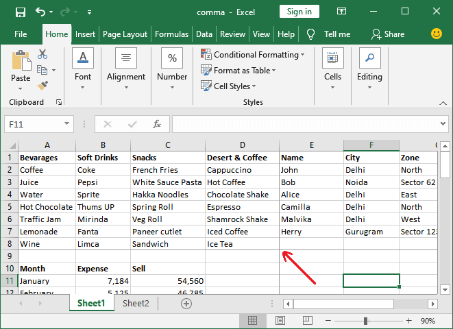
Horizontal page break inserts solid line just below to the selected row-cell. We will use the same Excel file that is used in the previous example.
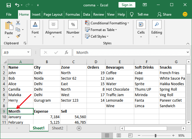
Step 1: To insert the Horizontal page break to your Excel spreadsheet, select the first cell of a row where you want to add a page break. For example, for 9th row, select the A9 cell.
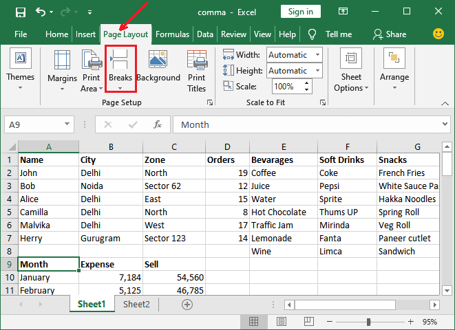
Step 2: Go to the Page Layout on the Excel menu bar, where you will get the Breaks option under the Page Setup section.
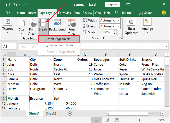
Step 3: Click on this Breaks dropdown button and choose Insert Page Break here.
Step 4: You can see that a solid grey line (Horizontal page break) has been inserted successfully above the selected cell in this Excel spreadsheet.
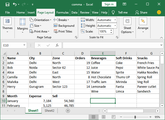
Press the Ctrl + P shortcut printing key to print preview the Excel sheet with page breaks how the data will get printed if after using horizontal page breaks.
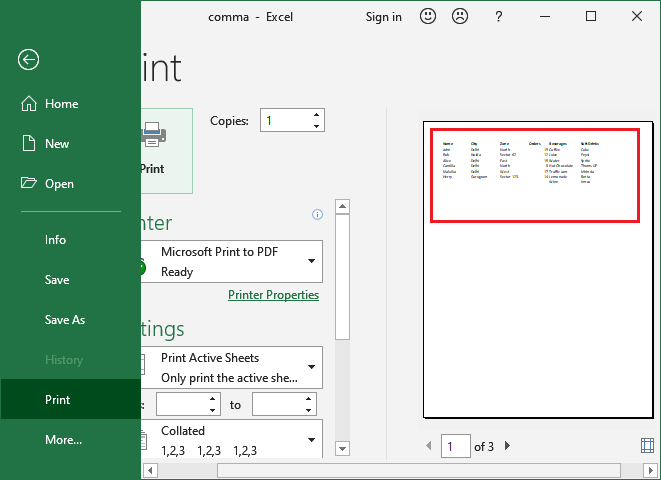
Here, in print preview, you can see that the Excel sheet has been from the selected row (horizontally but not vertically).
Vertical page break
Now, we will apply the vertical page break to this Excel table to get the needed print result. Vertical page break inserts dashed line previous to the selected column-cell. To insert the vertical page break to your Excel spreadsheet, follow the steps below:
Step 5: Select the first cell of the column from where you want to break the table data. For example, for E column, select the E1 cell.
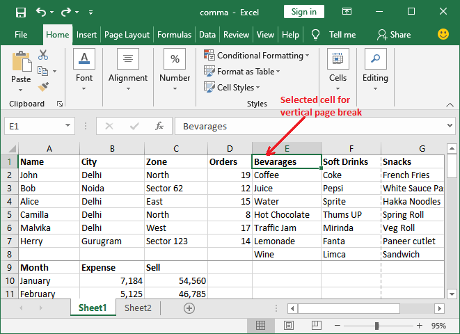
Step 6: In the Excel menu bar, go to the Page Layout tab, where you will get an option named Breaks under the Page Setup section.
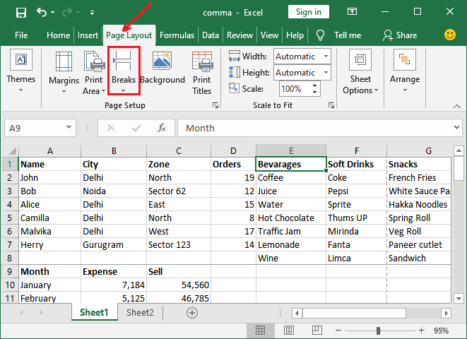
Step 7: Click on this Breaks dropdown button and choose Insert Page Break here.
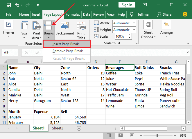
Step 8: You can see that a dashed grey line (vertical page break) has been inserted next to the selected column-cell successfully.
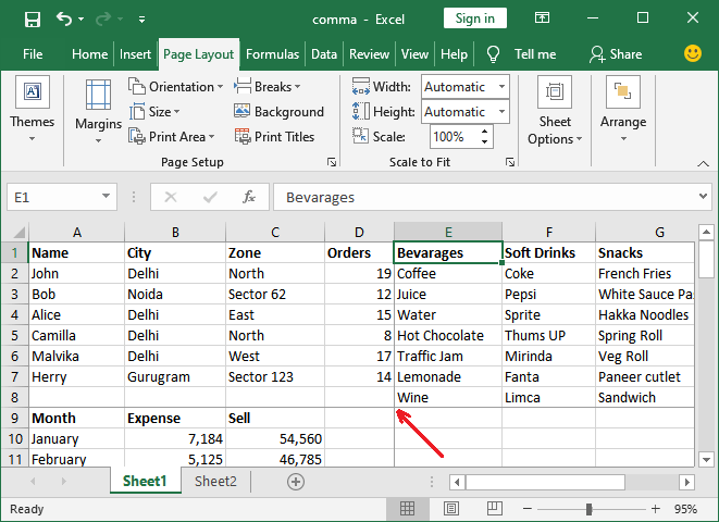
Now, press the Ctrl + P shortcut printing key to print preview the Excel sheet with page breaks how the data will get printed if after using horizontal page breaks.
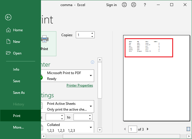
You can see that the data till the D column is displaying here because of the vertical page break. So, this is the main purpose of using page break in an Excel file.
2. Insert a page break using Page Preview
This is another way to insert a page-break to your Excel worksheet from the page preview method by right-click. In the Excel ribbon, you will find a Page Preview option inside the View menu. From here, you can preview the page break to your Excel worksheet.
Step 1: Open your Excel sheet in which you want to insert the page break. We have this worksheet.
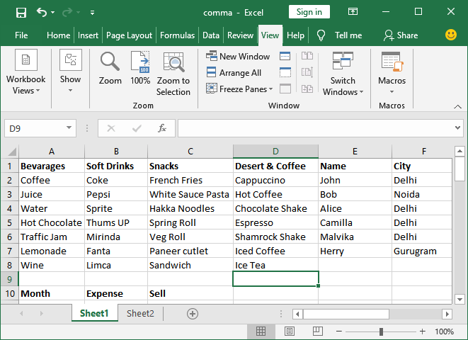
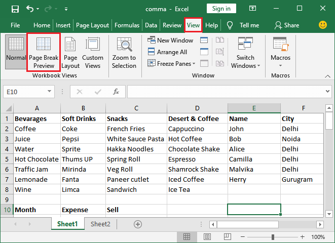
Step 2: Navigate to the View tab in the Excel menu bar where you will get the Page Break Preview option; click on it.
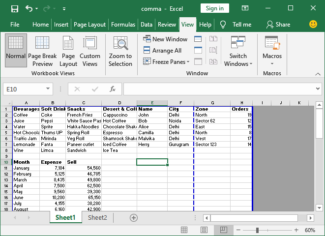
Step 3: This Page Break Preview option will show you a preview of your Excel sheet data in a grid. Here, blue lines define the edges of the page.
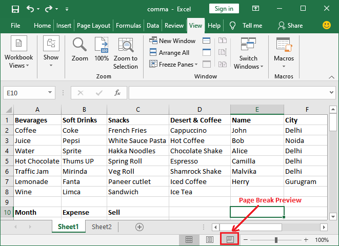
Note: You can also directly get this Page Break Preview option in the status bar at the bottom left side.
Step 4: Now, insert the page break to your sheet either horizontally or vertically. We will show you both.
Vertical page break
This time, we will insert the vertical page break first then the horizontal page break. Follow the steps below:
Step 1: Select the first cell of the column where you want to insert a vertical page break.
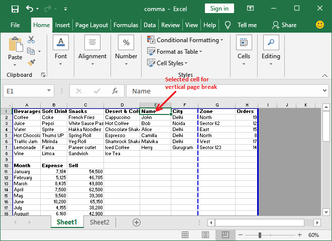
Step 2: Right-click your mouse/touchpad on that selected cell and Choose Insert Page Break from this list.
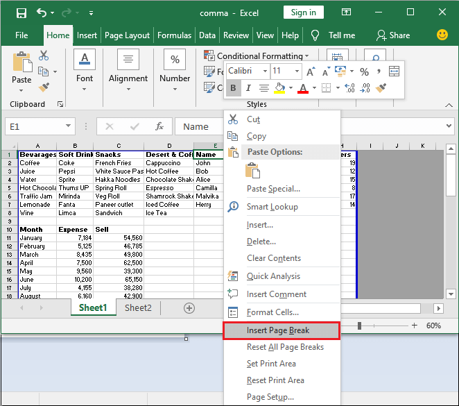
It will add a page break previous to the selected cell column automatically.
Step 3: In preview mode, you can see that where a solid line added vertically before the selected column cell. See in the screenshot below:
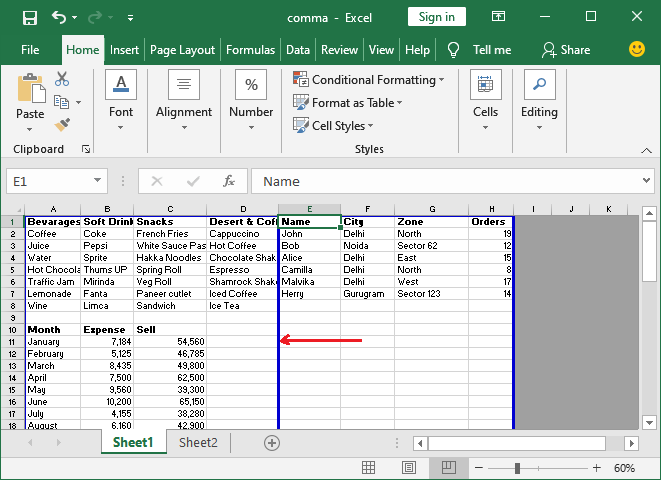
Step 4: Press the Ctrl + P shortcut printing key to print preview the Excel sheet with page breaks how the data will get printed if after using vertical page break.
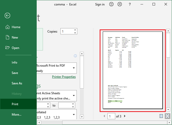
Here, in print preview, you can see that all the columns after the page break (solid blue line) have been removed from the table only while printing.
Step 5: You can exit from this page break preview mode by clicking on the Normal mode button present previous to the Page Break Preview option.
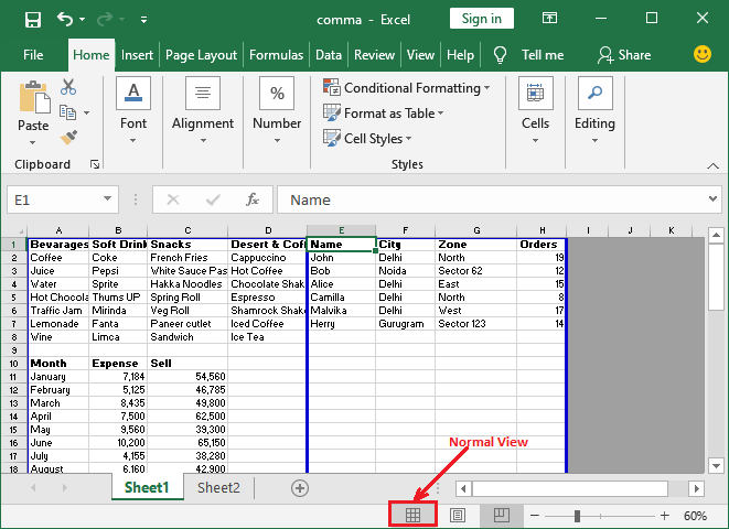
Step 6: It will take you to the normal Excel worksheet but with your added page breaks.
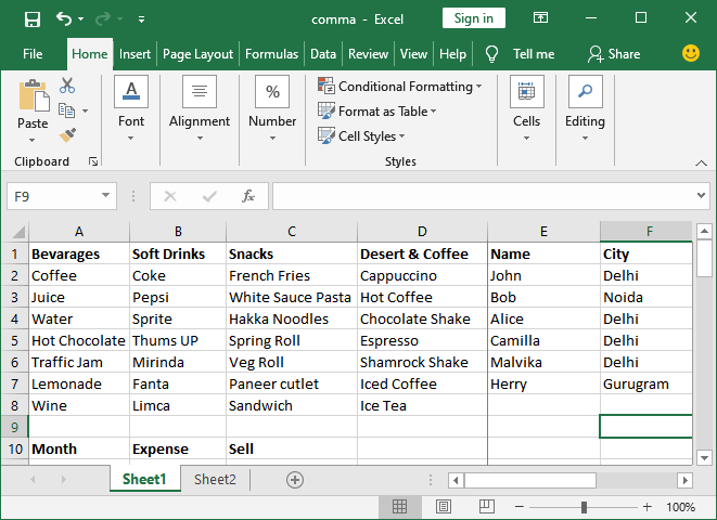
Horizontal page break
Now, we will insert a horizontal page break to the Excel worksheet by using the Page Preview method. For this, you have to enable the Page Break Preview mode again if you are in Normal View currently.
Step 1: From the bottom right corner, you can enable Page Break Preview mode by clicking on this button.
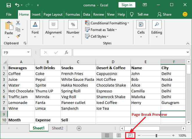
Step 2: Now, select the first cell of the row where you want to insert the horizontal page break. For example, select the A9 cell for 9th row.
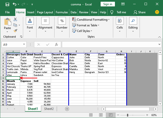
Step 3: Right-click your mouse/touchpad and select Insert Page Break from this list. It will add a page break above to the selected cell row automatically.
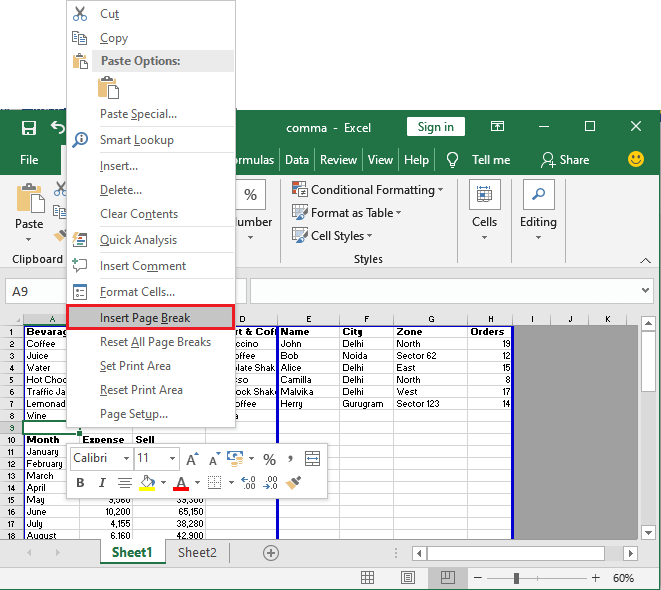
Step 4: See that a page break has been added horizontally in the Excel file just above the selected cell. See in the screenshot below:
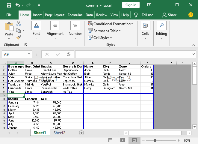
Step 5: Now, press the Ctrl + P shortcut printing key to print preview the Excel sheet with page breaks how the data will get printed after using page breaks (vertical and horizontal).
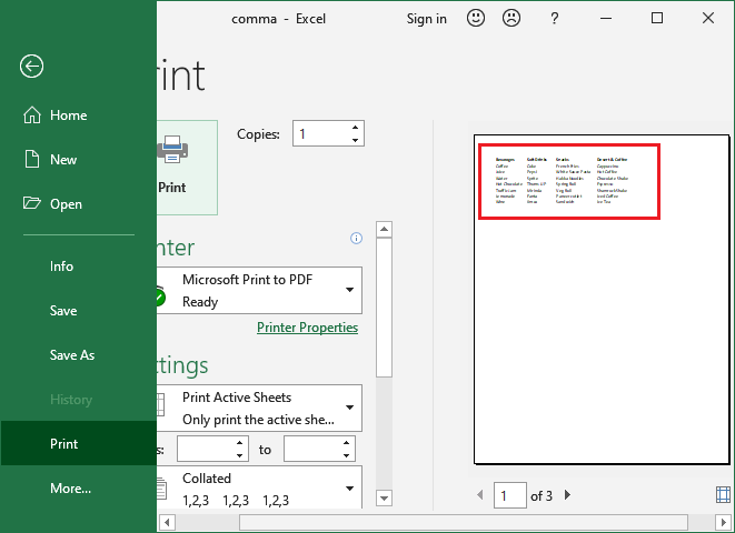
You can see that the data till the D column and 8th row is displaying here because of vertical page break and horizontal page break. Other data of this Excel sheet has been moved to the next page of the Excel sheet.
Step 6: Now, exit from the preview mode by clicking on the Normal option and see the normal Excel worksheet with your added page breaks.
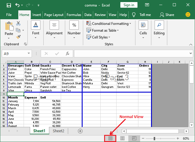
Step 7: After exiting from the Page Break Preview mode, the Excel sheet will visible normal and clear with your added page breaks that you inserted into your Excel sheet.
