How To Create A Chart With Floating Bars
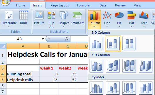
1. Consider the data set for chart.

2. Select all the data set. Go to the ribbon. Click Insert and in Column option select 2D Stacked Column.

3. Then a chart window will appear like below. Now for make it floating bars chart, right click on the lower shaded part. Select Format Data Series option.

4. On selecting data series option, a window will appear like this below. Choose Fill option from left hand side and select No Fill.

5. After step 4 the bars in the chart window become floating bars like shown in fig below. Now in tool bar under Layout option select Data Labels. Choose Center.

6. Here you go with the chart with floating bars. You can use is for timeline presentations about some process results. It looks much better when values increasing like in the example below.

Template
Further reading:
Basic concepts
Getting started with Excel
Cell References


