Consolidation

For starters, it is noteworthy that the tables are not identical and there are even different sizes. This is not an obstacle to their consolidation. Consolidation of the sales table in Excel start with ribbons. Required Consolidate button located in the Data tab.

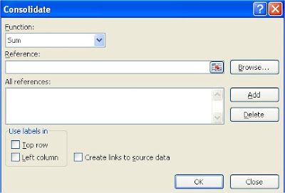
Select the location where you want the summary table and click Consolidate. You get the following dialog box:

You can select up to 11 different functions for data consolidation. You just want to summarize data, so we choose Sum. The tables contain the label in the top row and left column, then select the appropriate check boxes in the dialog box. Select a check box with which you will see a link to the source data. This is a very useful option, which will facilitate analysis of data in the summary table.

Now, add references to tables. Click on the button and add each of the tables turn.

Consolidation is ready. All data are summed up individually and have created a summary table. The result looks like this:

On the left side shows the digits 1 and 2 and pluses. We also see that the individual lines are not in sequence as if some rows were hidden. This is precisely the result of the creation of links to the source data. The data source table have been grouped and summarized in the table you created. 1 and 2 are different levels of detail table. After clicking on the two show up all the individual data including those from the source table. As you can see it developed all the pluses on the left side of the table.

There were individual data from all the consolidated table and file name. If you do not need as this level of detail, you can develop only a plus, eg. sales data Salesman2.

By consolidating data in a simple way you can work with data in Excel. Consolidate data most likely to be useful in the preparation of reports or periodic data aggregation.

Further reading: 
What-If Analysis
How Excel handles different data types?