Excel Exact Function
When analyzing large chunks of Excel data, you often need to match the exact value of some data with another. Microsoft Excel has a special function to compare two strings and states whether they are an exact match or not, the Exact function. It is a case-sensitive function that compares two text values and returns Boolean True or False.
In this tutorial, we will have a closer look at EXACT function and will learn the step by step procedure to apply this function in your Excel worksheet.
What is an EXACT function?
The Microsoft Excel EXACT function compares two strings and returns TRUE if both values are the same. Otherwise, it will return FALSE. This function is case-sensitive.
The EXACT function is a built-in function that can be used as a worksheet function (WS) in Excel. As a worksheet function, the EXACT function can be entered as part of a formula in a cell of a worksheet.
This function falls under Excel String/ TEXT functions. The EXACT function assists the user in checking whether the specified two text or string values are exactly equal (including the cases) or not. If they are equal and give a 100% match, this function returns Boolean TRUE. Otherwise, it returns FALSE. The EXACT is a case-sensitive function that means “CAT” and “cat” will be considered differently as one is in uppercase and one in lowercase.
In financial jobs, you often need to examine and compare two values while analyzing the data. In such a situation, the EXACT function supports you to do the comparison easily. This function also becomes handy when sharing our workbooks with others and letting them input the data in a specific format.
NOTE: The EXACT function is case-sensitive when it compares the two strings.
Syntax
Parameter
- Text1 (required): This argument specifies the first string for which you want to check the exact match.
- Text2 (required): This argument specifies the second string which you want to test against.
Return
- The EXACT function returns Boolean TRUE if both the parameters (text1 & text2) are the same.
- The EXACT function returns Boolean FALSE if both the parameters (text1 & text2) are different.
Points to Remember for Exact function
- The standard equals to (=) operator is not case-sensitive.
- EXACT can only compare and finds the match for string values. It you pass numeric values in its parameter it converts them to text.
Example 1: Testing condition 1 and condition 2 to check the numbers are greater than 0 using Excel EXACT function.
| Col A | Col B | Exact Result |
|---|---|---|
| EXCEL | EXCEL | |
| Fill | FILL | |
| GREAT | GREAI | |
| Match | Match |
To check whether Col A is an exact match of Col B or not follow the below given steps:
STEP 1: Insert a helper column
Add a column next to “Col B” and type the column name “Exact result” on top of the cell.
It will look similar to the below image:
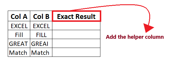
In the helper column, we will type the EXACT function for every row and check whether Col A is an exact match of Col B.
NOTE: As the above image shows, we have formatted the column with borders and font to make the worksheet more visually attractive.
STEP 2: Insert the EXACT formula
The next step is to enter the formula so put your cursor in the second row of your helper column start typing: = EXACT(
It will look similar to the below image:
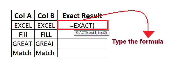
STEP 3: Add the parameters
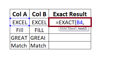
- The first parameter includes “Text1” which represents the first string that you want to check. Here, cell reference B4 holds our Text1. So our formula becomes: =Exact(B4,
It will look similar to the below image:
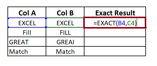
- The first parameter includes “Text1” represents the first string which you want to check for the exact match. Here, cell reference C4 holds our Text1. So our formula becomes: =Exact(B4,C4)
It will look similar to the below image:
STEP 4: EXACT will return the result
EXACT (B4, C4) will return the Boolean TRUE as a result because the values in both the columns (EXCEL, EXCEL) are in uppercase and are getting matched.

STEP 5: Drag the formula to other rows to repeat
Put your cursor on the formula cell and take it towards the right of the rectangular box. You will notice that the cursor will change into the ‘+’ icon.
It will look similar to the below image:

Drag the + icons to all the cells below it. This will automatically copy the EXACT function to all the cells. As a result, EXACT will return Boolean TRUE if both the string matches and false if it doesn’t.
Refer to the below image for the output:
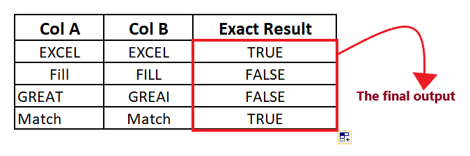
NOTE: In the above example, the result of the second and third row is FALSE because the EXACT function is case-sensitive. In the second row, the first value is an upper case combination of the upper and lower case, whereas the second value is in the upper case.
Example 2: Using the Exact function calculate the product (soft toys) details from the below given table and find its revenue for the year.
| Products | Revenue |
|---|---|
| SOFT TOYS | 200 |
| soft toys | 400 |
| creative toys | 320 |
As shown in the above table, we have two values named with soft toys with the only difference that one is in lowercase (soft toys) and the other value in uppercase (SOFT TOYS). But we want the lowercase data value “soft toys”. However, there are other Excel functions such as VLOOKUP and INDEX/MATCH to look for the given values, but the only problem is that it is not case-sensitive. So, we will use a combination of “SUMPRODUCT + EXACT” to achieve a case-sensitive lookup.
Follow the below-given steps to product details and revenue for soft toys:
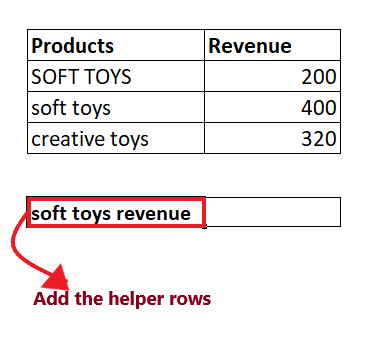
STEP 1: Insert a helper row named “soft toys revenue”
Place your cursor anywhere under products table and type the row name “soft toys revenue” on top of the cell.
It will look similar to the below image:
In the helper column, we will type the combination of the SUMPRODUCT + EXACT function to find the revenue details.
STEP 2: Insert the SUMPRODUCT formula
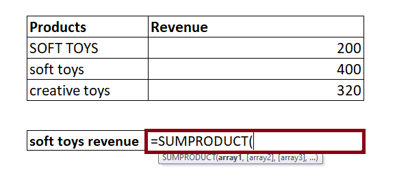
- The next step is to enter the formula so put your cursor in the second row of your helper column start typing: = SUMPRODUCT(
It will look similar to the below image:
NOTE: Excel SUMPRODUCT function returns the sum after multiplying numbers in an array, and it can also be used to count cells based on the criteria provided. This function takes arrays as its parameters.
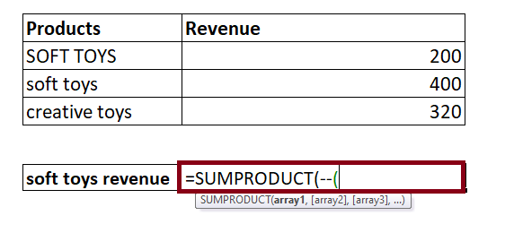
- Before inserting the parameters, add two negative signs. We have used a double negative to convert the output TRUE & FALSE values to 1’s and 0’s. So our formula becomes: =SUMPRODUCT(–(
Refer to the below image:
STEP 3: Insert the EXACT function as the first parameter of SUMPRODUCT
- In the first parameter, we will type the EXACT function. So our formula becomes: =SUMPRODUCT(–(EXACT(
- Next, we will pass the parameters of EXACT. In the first parameter, we will pass the string which you want to check. Here, cell reference B4 holds our Text1. So our formula becomes: =SUMPRODUCT(–(EXACT(B5,
- In the next parameter, we will pass the products name from which you want to test against. So our formula becomes: =SUMPRODUCT(–(EXACT(B5, B4:B6)
It will look similar to the below image:

STEP 4: Insert the second parameter of SUMPRODUCT
Enter the revenue range as the second parameter of SUMPRODUCT. Here, cell range C4:C6 holds the revenue range. So our formula becomes: =SUMPRODUCT(–(EXACT(B5,B4:B6)),C4:C6).
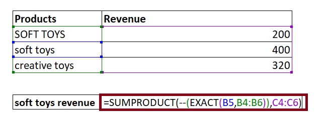
STEP 5: Combination of Excel SUMPRODUCT and EXCAT function will return the result
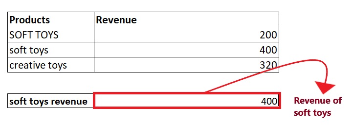
EXACT will return the output for the formula after running a test on the values in column B, convert the TRUE/FALSE (output of the EXACT function) to 1’s and 0’s. As shown below, using the combination of SUMPRODUCT and EXACT, you will have the revenue for ‘soft toys’ product.
Eureka! Now you have successfully covered all the steps and examples for the EXACT function. Go ahead, use it whenever you need to do any comparison, combine it with other functions and fetch satisfactory results.


