How to do addition in Excel

One of the typical day-to-day operations performed in Excel is addition. Whether you have to find the sum of the price list, expense sheet, and calculate the total sales or any other action. You can even create your customized SUM formulas by combining the SUM function with other Excel functions.

Therefore, in this tutorial, we will cover the various ways to quickly calculate the sum of numbers in excel.

1. Sum a column in Excel with one click

This is one of the fastest options that is quickly used to find the sum of numbers. To apply this method, follow the below steps.

1. Click on the column alphabet for which you want to find out the sum.
2. At the Excel Status bar, you will notice the total of the cells.
   
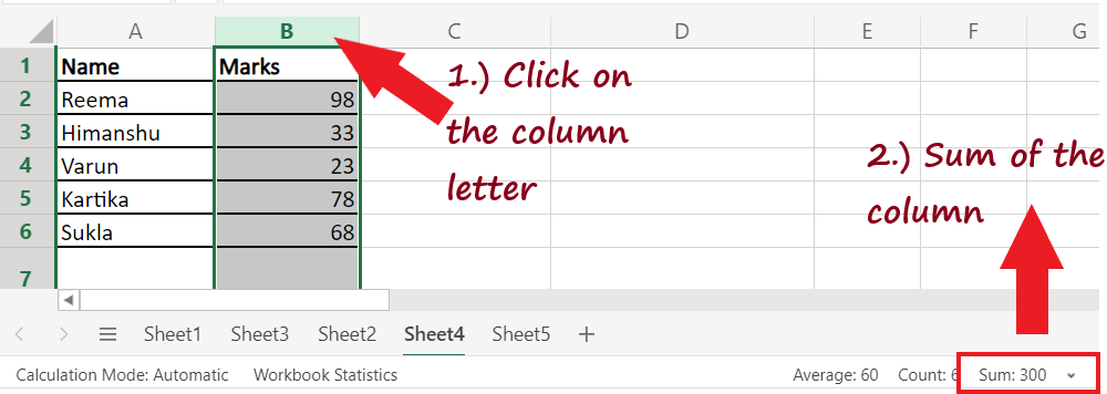
3. Instead of selecting the entire column, you can select a few cells to calculate the sum. It will quickly display the sum of the selected cells in the Excel status bar.

NOTE: Though this method is quick, the drawback of this method is that it neither allows copying nor shows numeric digits.

2. Calculate the sum in Excel with AutoSum

The second method down in your list is AutoSum. This method allows the user to quickly sum up a column and hold the output in the table. The advantage of using the AutoSum method is that it automatically adds up the numbers and will present the result in the specified cell. To apply this method, follow the below steps.

1. Click on the empty cell below the column where you want to sum up the numbers.

NOTE: To bypass any additional operations like range selection, always select the first empty cell below the column you require to sum.

2. Go to the Home tab -> Editing group -> AutoSum option.

3. Excel will automatically pick the range and will put the same in the SUM function. Though if needed, you can alter the range as well.

4. Click on the Enter button on your keyboard, and you will notice Excel will immediately give you the sum of the numbers present in the selected range.

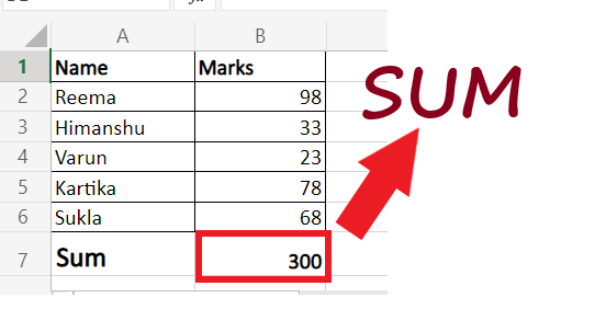
This method is fast and lets you automatically get and keep the summing result in your table.

3. Addition using the SUM function

One of the easy methods commonly used to find the total in Excel is the SUM function. The SUM function is used to select specific cells or even a large range in an Excel worksheet and calculate their total. This method is beneficial if you have a large excel column and want to calculate the sum without highlighting the range. Though, you still need to enter the SUM function manually.

NOTE: The SUM function calculates the sum of all the values selected in the range even if the cells are hidden or filtered.

Using the SUM function in Excel, you can find a range of cells, an entire column/row, contiguous cells, or even non-contiguous cells. Excel users often create customized advance functions by combining the SUM function with other Excel functions.

To apply this method, follow the below steps.

1. Click on the empty cell below the column where you want to sum up the numbers.

2. Start the formula with equal to (=) followed by SUM (). In the arguments select the range of the cells by pointing your mouse to one cell and dragging the cursor to the end. If you want you can directly enter the number of cell references separated by comma.

NOTE: You can also manually type the SUM range address. It is helpful to calculate large range data easily. For example =SUM(D2:D3000).

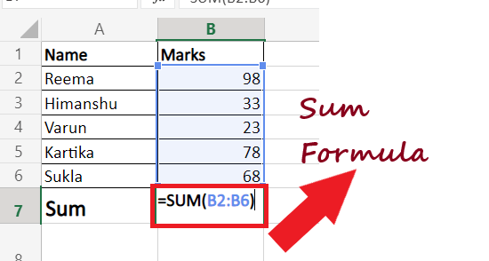
3. Press the Enter button and Excel will immediately calculate the sum of numbers.

4. Find Sum of only visible cells

In the above section, we have covered that SUM functions add all the values, including the hidden and filtered fields. Therefore, with this method, we learn how to calculate the sum only for the visible cells. Therefore, omitting the filtered or hidden cells. To apply this method, follow the below steps.

1. Enter your data in Excel spreadsheet.
   
2. Now, we will filter the above dataset and fetch only the values that are greater than 40. Click on any cell and go to Data-> Sort & Filter-> Filter icon.
   
3. As shown below the filter arrows will appear in the header. Click on the Marks filter arrow.
   
4. The following window will appear. Click on Number Filters-> Greater than.
   
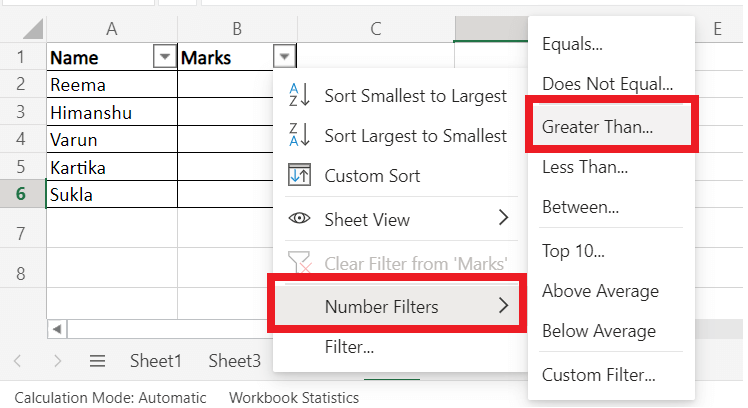
5. It will display the Custom Filter window. In the textbox, type 40 and press ok.
   
6. It will show you the following filtered output.
   
7. To quickly find the sum of the filtered column, select the range and click on AutoSum under the Home tab. You will have your filtered sum in the selected cell.
   
8. Another method to quickly find the sum is by selected the filtered cells and view the sum of the cells on the Excel Status bar. Though with this method, you won’t be able to paste the data into your worksheet.

5. Convert data into Excel table and get the sum for your column

Creating tables and calculating the sum of the columns is also one of the common methods to find the sum. Therefore if you have a large dataset and want to find the sum, convert your data to Excel Table. It will be helpful to quickly total the sum of the columns and rows of your table. To apply this method, follow the below steps.

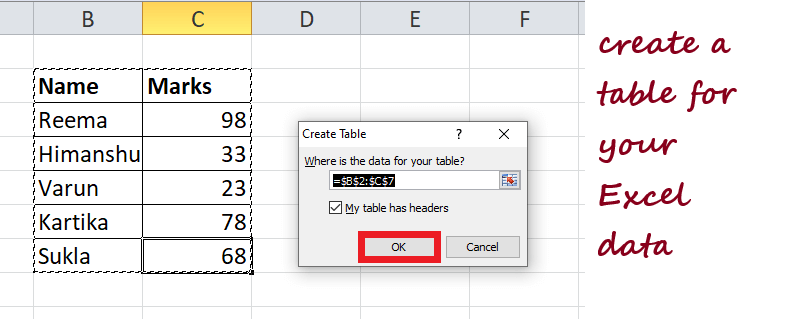
1. Put your cursor on any cell and press the shortcut key’ Ctrl + T’ on your keyboard to create a table out of your Excel data. You will have the given Create Table window and it will automatically select the data for you. Click on OK.
   
2. Excel will create a table for you. Next, in the ribbon toolbar, you will see the Design tab. Navigate to this tab and look for the Total Row. As shown below, tick the checkbox given in front of the Total Row.
   
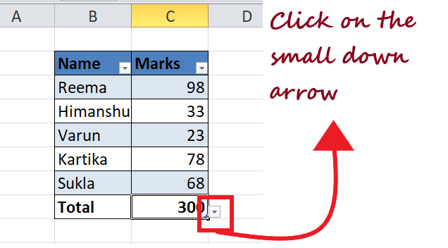
3. Excel will immediately add a new row (named with Total) at the end of your table. Though it already calculates the sum, still make sure to click on the small arrow icon next to your number.
   
4. Select the SUM option from the appeared options. That’s it you will get the sum of your data.
   
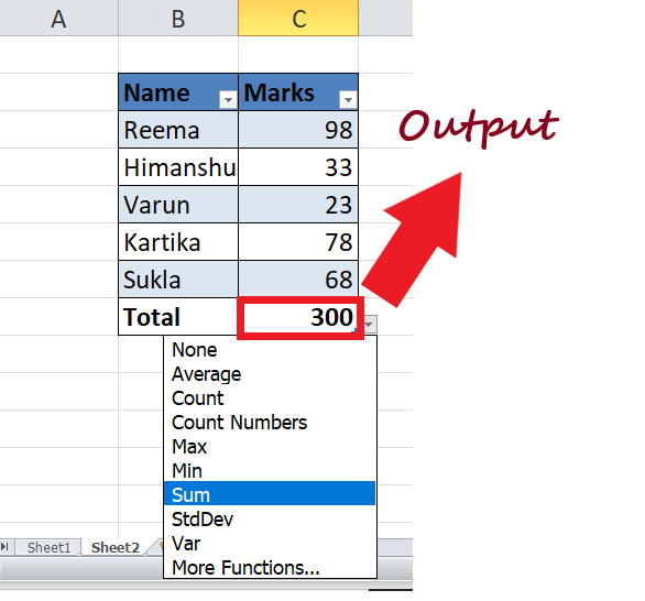
5. Using the method you can easily find the sum of every column. You can also try the other options as well such as Average, Min and Max.

NOTE: This method also adds up only the visible (filtered) cells.