Excel Large Function
Many times while working with Excel worksheets, you need to find out the largest number or sometimes the 5th largest number in your data series. While you may think of applying Excel formulas, but the easier way to get it solved it by using the inbuilt Excel LARGE function.
What is Excel LARGE Function?
The Excel LARGE function is used to return a numeric value based on its position in a specified list where the list is sorted by value arranged in descending order. In simple words, LARGE can fetch the “nth largest” value, unlike the 1st largest value, 2nd largest value, 3rd largest value, and so on.
The LARGE function is completely automatic – you only need to provide the range of data values and an integer for “nth” to specify the ranked value you want and it will return the nth largest number from the specified range of values. For example, the LARGE function is useful when you want to retrieve the first, second, or third highest scores for a match. The LARGE function comes under the category of Excel Statistical functions.
Syntax
Parameters
- Array (required): This parameter represents the list of numbers from which you want to find out the nth largest number.
- nth largest number (required): This parameter represents the nth largest number which needs to be found out for example 8th largest number etc.
Return
This function returns the nth largest number from the given set of values.
Points to Remember
- The LARGE function evaluates only numeric data and it ignores blank cells, text values, and logical (TRUE and FALSE) values.
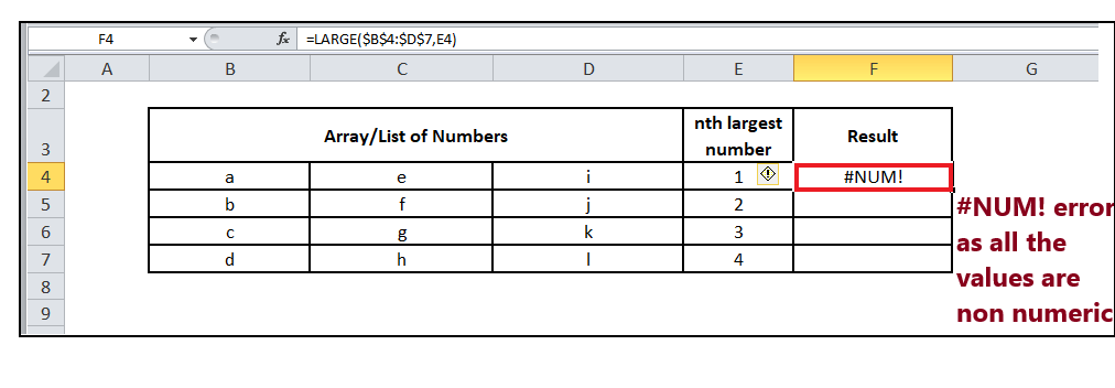
- If the array parameter contains non numeric data, LARGE function returns the #NUM! error.
- Sometimes users use the LARGE function to determine the rank of a number. But it won’t work. To find the rank of a number in a data set, use the RANK function.
Examples:
Example 1: Use LARGE function to find the nth LARGE value from the set of values in the range A18:C21.
| Array/List of Numbers | nth largest number | ||
|---|---|---|---|
| 3 | 1 | 5 | 1 |
| 19 | 50 | 1 | 5 |
| 8 | 12 | 20 | 4 |
| -8.5 | 3 | 0.5 | 12 |
To find out the smallest nth value follow the below given steps:
STEP 1: Add a helper column named Result
Put your mouse cursor to the cell next to “nth largest number” and Type result on top of it.
It will look similar to the below image:
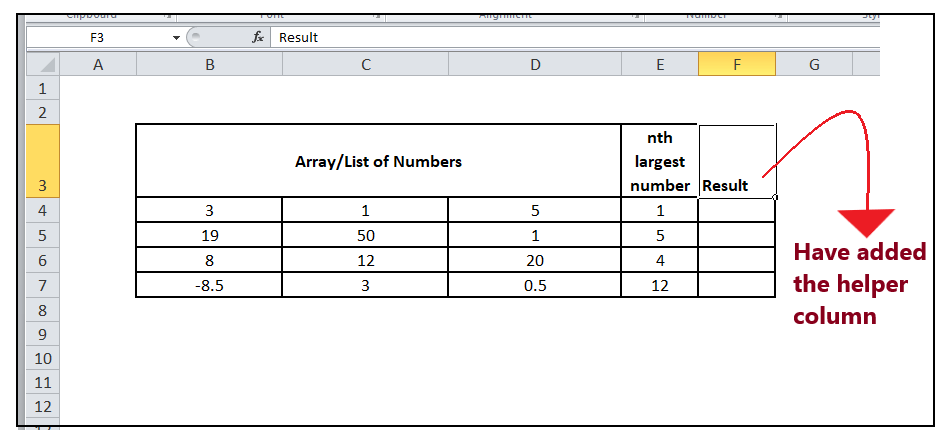
In this column we will enter the formula and will find out the nth LARGE value of various numeric data values.
NOTE: You can also format this column unlike others to make your Excel worksheet more visually appealing.
STEP 2: Insert the formula
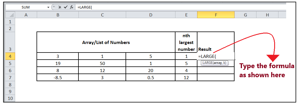
Move to the second row and start typing the formula = LARGE(
It will look similar to the below image:
STEP 3: Add the parameters
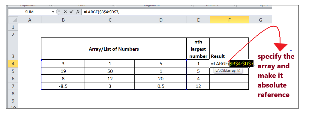
- The first parameter represents the input array of the nth LARGE value you want to calculate. So, the range is B4:D7, which includes the list of numbers.
- Use absolute References for the array range. Select the array range and press F4 and the value given for array will be converted to the absolute reference i.e., $B4:$D7.
It will look similar to the below image:
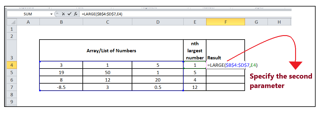
- In the 2nd parameter, you are required to specify the nth largest number that you want to find. Here, we have specified cell D4.
It will look similar to the below image:
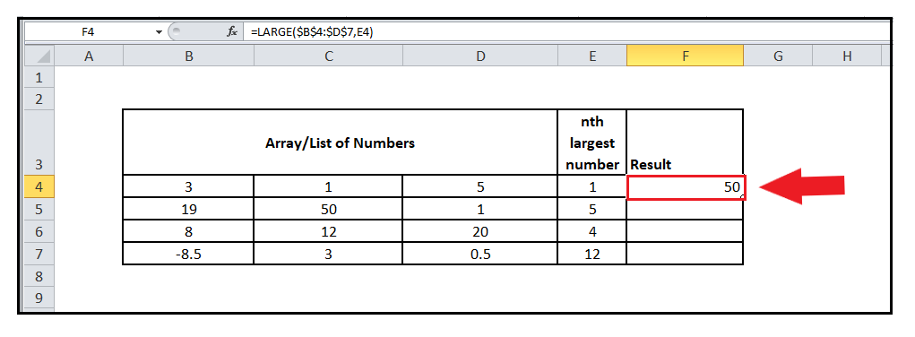
STEP 4: LARGE will return the result
The LARGE (C4: C11, D4) will return the first largest number as 50.
STEP 4: Drag the formula to other rows to repeat
Put your cursor on the formula cell and take it towards the right of the rectangular box. You will notice that the cursor will change into ‘+’ icon.
It will look similar to the below image:
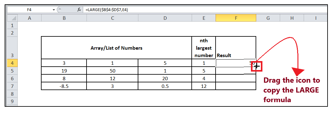
Drag the + icons to all the cells below it. This will automatically copy the LARGE function to all the cells. Notice in the above formula the columns are locked (as we made them absolute reference), but rows are not. This enables the Excel rows to update as the formula is copied down, allowing it to change as the formula, but prevents the array from changing as the formula is copied across.
Refer to the below image:
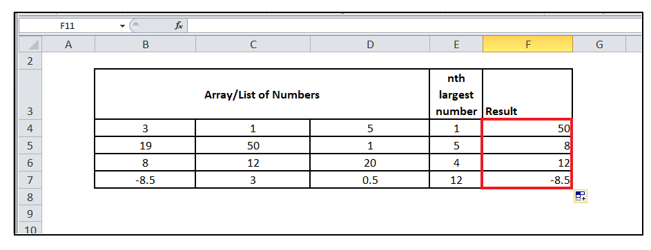
You will get the 1st largest value, 5th largest value, 4th largest value, and 12th largest value, from the specified range of data set.
Example 2: Calculate nth largest number for the following numbers
| Array/List of Numbers | nth largest number | ||
|---|---|---|---|
| 3 | 5 | 3 | 1 |
| 19 | 2 | 1 | 2 |
| 8 | 5 | 3 | 3 |
| 1.5 | 1 | 4.5 | 4 |
To find out the smallest nth value follow the below given steps:
STEP 1: Add a helper column named Result
Put your mouse cursor to the cell next to “nth largest number” and Type result on top of it.
It will look similar to the below image:
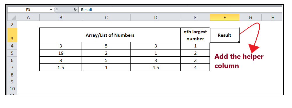
In this column we will enter the formula and will find out the nth LARGE value of various numeric data values.
NOTE: You can also format this column unlike others to make your Excel worksheet more visually appealing.
STEP 2: Insert the formula
Move to the second row and start typing the formula = LARGE(
It will look similar to the below image:

STEP 3: Add the parameters
- The first parameter represents the input array of the nth LARGE value you want to calculate. So, the range is B4:D7, which includes the list of numbers.
- Use absolute References for the array range. Select the array range and press F4 and the value given for array will be converted to the absolute reference i.e., $B4:$D7.
- In the 2nd parameter, you are required to specify the nth largest number that you want to find. Here, we have specified cell E4.
It will look similar to the below image:

STEP 4: LARGE will return the result
The LARGE (C4: C11, D4) will return the first smallest number as 19.
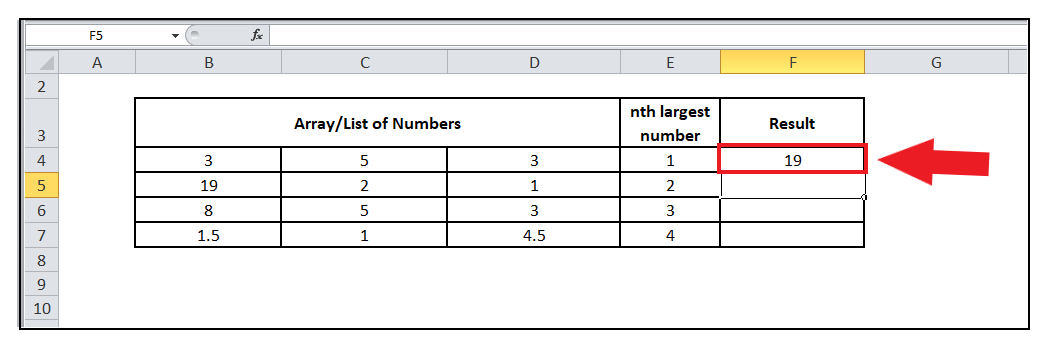
STEP 4: Drag the formula to other rows to repeat
Put your cursor on the formula cell and take it towards the right of the rectangular box. You will notice that the cursor will change into ‘+’ icon.
Drag the + icons to all the cells below it. This will automatically copy the LARGE function to all the cells. Notice in the above formula the columns are locked (as we made them absolute reference), but rows are not. This enables the Excel rows to update as the formula is copied down, allowing it to change as the formula, but prevents the array from changing as the formula is copied across.
Refer to the below image:
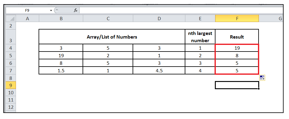
You will get the 1nd largest value, 2nd largest value, 3rd largest value, and 4th largest value, from the specified range of data set.
Example 3: Calculate nth largest number for the following text
| Array/List of Numbers | nth largest number | ||
|---|---|---|---|
| a | e | i | 1 |
| b | f | j | 2 |
| c | g | k | 3 |
| d | h | l | 4 |
To find out the rank of race results follow the below given steps:
STEP 1: Add a helper column named Rank and insert the formula
- Put your mouse cursor to the cell next to “nth largest number” and Type Result on top of it.
- Move to the second row and start typing the formula = LARGE(
It will look similar to the below image:
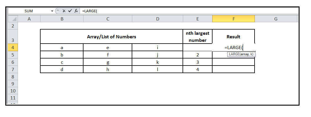
STEP 2: Add the parameters
- The first parameter represents the input array of the nth LARGE value you want to calculate. So, the range is B4:D7, which includes the list of numbers.
- In the 2nd parameter, you are required to specify the nth largest number that you want to find. Here, we have specified cell E4.
It will look similar to the below image:

STEP 3: Excel will throw #num! Error
This function is specifically made to fetch the nth largest number for numeric data values, but if the specified data range contains all non-numeric values, it will throw an error. Since in our case as well all the data values are non-numeric, therefore Excel has thrown #num! error stating that there is a problem with the array of numbers used in the function.
