How to Search in Excel?
There are multiple ways to search in Excel. The first option is to find a particular piece of data in a cell or group of cells among a massive spreadsheet.
The second option includes using search functions like VLOOKUP or HLOOKUP that let you search one sheet for data and output the results in a second cell location or a different worksheet.
Most of the time, searching in an Excel spreadsheet is easy. If you can’t scan through the rows and columns, you can use Ctrl + F to open a search dialog box. If you’re working with a really big spreadsheet, it can save a lot of time to use one of these four lookup functions.
How to Search Using the Search Sheet Bar
Follow the following steps to search specific data in excel by using the search sheet bar.
Step 1: Click into the taskbar with the faint words “Search Sheet” at the top right corner of the spreadsheet and enter the words or numbers which you want to search in the sheet.
Step 2: Press Enter or Return if you’re using a Mac to find the data. And then use the arrows beside the search term to jump to the next or previous data.
Step 3: Also, you can quickly access this search bar by using a “command + F” keyboard shortcut on a Mac and a “Control + F” shortcut on a PC.
How to Search Using Find Feature
With Excel open to your spreadsheet with data, you can find anything on the spreadsheet using a straight word search or using special wildcard characters. Follow these steps to use the find feature in Excel:
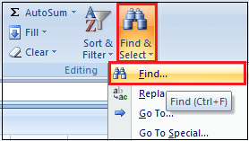
Step1: Go to the Home tab. And select Find & Select button in the Editing group, then select the Find feature.

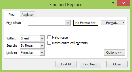
Step 2: You’ll see a simple Find and Replace window. Also, you can see all of the advanced options by selecting Options.

You can use the following options to fine-tune your search:
- Find what: Type the text or number that you want to find in the worksheet.
- Format: Select this button to only search for text with the formatting you define in the Find Format window.
- Within: Select Sheetor Workbook to search inside the current sheet or across the entire workbook.
- Search: Select By Rowsor By Columns to conduct your search a row at a time or a column at a time (and stop on that row or column when it finds a result).
- Look in: You can deepen your search to other areas of your spreadsheet by telling the search to look in Formulas, Values, Notes, or Comments.
- Match case: This will search using case-sensitive text matching.
- Match entire cell contents: This will search for cells that only contain the text you type.
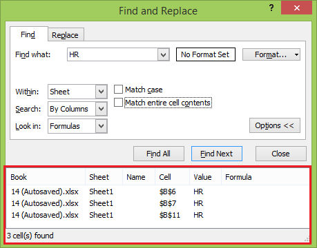
If you select Find Next button, you’ll see each incident in the spreadsheet where the text is found highlighted. Select the button again to move on to the next result. If you want to see them all at once, select the Find All button.
Step 3: This displays all of the results, along with the sheet and cell number where they’re found, in a list at the bottom of the window. Just select any one of them to see that cell in the sheet.

Excel Search Wildcard Characters
When you’re typing search characters into the Find What field, you must understand how wildcard characters work. These let you customize more advanced search so you can search in Excel and find exactly what you’re looking for in the worksheet.
- Question mark (?): Replace any single character or number. For example, type c?t to find any three-letter word that starts with c and ends with t, such as cat, cut, or cot.
- Asterisk (*): Replace parts of words. For example, type c*tto find any length word from cart and cast to count and court.
- Tilde (~): Use this character to override the special characters above. For example, if you want to find the word “user?” including the question mark, you can type user~?and this will override the special ? character to search, including the question mark.
Excel SEARCH Function
The SEARCH function in Excel is very similar to the FIND function. It also returns the location of a substring in a text string. Unlike FIND, the SEARCH function is case-insensitive, and it allows using the wildcard characters.
Syntax
Below is the basic syntax of the SEARCH function.
Example
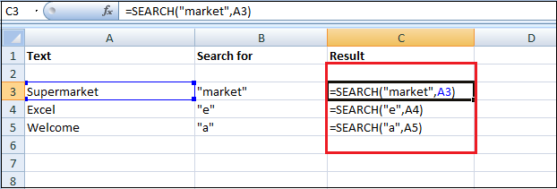
And here are some examples to evaluate the search function.
=SEARCH(“market”, “supermarket”) returns 6 because the substring “market” begins at the 6th character of the word “supermarket”.
=SEARCH(“e”, “Excel”) returns 1 because “e” is the first character in the word “Excel”, ignoring the case.

Like the FIND function, Excel’s SEARCH function also returns the #VALUE! Error if:
- The value of the find_text argument is not found.
- The start_num argument is greater than the length of within_text.
- Start_num is equal to or less than zero.
How to Search Using Functions
In Excel, Many useful functions let you search columns, rows, or tables to find information and return related information.
The following are a few examples of the most popular functions you can use to search in Excel.
1. VLookup Function
This function allows you to specify a column and a value. It will return a value from the corresponding row of a different column. Here’s the syntax of the function:
- [lookup_value]is the piece of information that you already have.
- [table_array]lets you specify the cells in which the function will look for the lookup and return values. When selecting your range, be sure that the first column included in your array is the one that will include your lookup value.
- [col_index_num]is the number of the column that contains the return value.
- [range_lookup] is an optional argument and takes 1 or 0. If you enter 1 or omit this argument, the function looks for the value you entered or the next-lowest number.
2. HLOOKUP Function
Where VLOOKUP finds corresponding values in another column, HLOOKUP finds corresponding values in a different row. Because it’s usually easiest to scan through column headings until you find the right one and use a filter to find what you’re looking for, HLOOKUP is best used when you have really big spreadsheets, or you’re working with values that are organized by time.
Here’s the syntax of the function:
- [lookup_value] is the value that you know and want to find a corresponding value for.
- [table_array]is the cells in which you want to search.
- [row_index_num]specifies the row that the return value will come from.
- [range_lookup] is the same as in VLOOKUP. Leave it blank to get the nearest value when possible, or enter 0 to only look for exact matches.
3. INDEX and MATCH Function
INDEX and MATCH are two different functions, but they can make searching a large spreadsheet a lot faster when they’re used together. Both functions have drawbacks, but by combining them, we’ll build on the strengths of both.
Below is the syntax of both functions:
- [array]is the array in which you’ll be searching.
- [row_number]and [column_number] can be used to narrow your search (we’ll take a look at that in a moment.)
- [lookup_value]is a search term that can be a string or a number.
- [lookup_array]is the array in which Microsoft Excel will look for the search term.
- [match_type]is an optional argument that can be 1, 0, or -1. 1 will return the largest value that is smaller than or equal to your search term. 0 will only return your exact term, and -1 will return the smallest value that is greater than or equal to your search term.
How to Search for Excel Formulas
In Excel, the search for formulas is a little different because formulas display numbers in a cell. It can be difficult to know which cells contain numbers and which cells contain formulas.
To help you find which cells contain formulas, Excel gives you two choices:
- Display formulas in your cells (instead of numbers).
- Highlight the cells that contain formulas.
And to display (or hide) formulas in a spreadsheet, you have two methods, such as:
Method 1: Press Ctrl + (an accent grave character, which appears on the same key as the ~ sign, often to the left of the number 1 key near the top of a keyboard).
Method 2: Click the Formulas tab, and then click the Show Formulas button in the Formula Auditing group.

This image shows what a spreadsheet looks like when formulas appear inside cells.

To highlight all cells that contain formulas, follow these steps:
Step 1: Go to the Home tab.
Step 2: Click on the Find & Select icon in the Editing group. And a pull-down menu appears.

Step 3: Then click on the Formulas. Excel highlights all the cells that contain formulas.

Difference between SEARCH and FIND Functions
In Excel, the FIND and SEARCH functions are very similar in terms of syntax and use. However, there are still some differences that distinguish them to be selective for solving query in Excel.
| FIND Function | SEARCH Function |
|---|---|
| The Find function is used to query a certain sub-string or character within a string and text stream. | The Search Function is used to getting the initial character of a sub-string or text in a string. |
The syntax used for querying a string with find function is shown as below:
Syntax: =FIND(find_text, within_text,[start_num]) |
The syntax for the SEARCH function can be described as given below:
Syntax: =SEARCH(find_text, within_text,[start_num]) |
| Use the Find function for an exact search of text. Confirm the sensitivity of the characters While using the Find function because it is a case-sensitive function. | The search function doesn’t differentiate between upper and lower case characters during a search because it is a case insensitive function. |
| The Find function does not allow the WildCard characters. | The Search function allows the WildCard characters, such as “*”, “?”.
|


