How to subtract time in Excel?
Subtracting a time from another time is a type of operation of calculating time difference. Time difference can be a useful operation of Excel. So, the user should know how to perform it.
Suppose that you have a task to complete within the given time period. Now, you want to know much hours work has been done from the total hours. You can find it by subtracting the work done hours from total hours.

You will learn the time manipulation operation in an Excel sheet with the help of this chapter. You will also explore the time functions offered by MS Excel.
How to calculate time difference?
Excel offers more than one formula to get the time difference. The users need start time and end time to calculate the time difference. Or, if they want to calculate the remaining time from the total assigned hours, they need the total assigned hours and how much hours work has been done.
To make the information more informative, you need to apply the formatting to your resultant value (time difference). The calculated time can be in hours, minutes, and seconds. You have to set in which format you want to get the time difference.
Custom time formatting
The custom time formatting can be applied to data from the Format cells dialogue box. Following are the basic codes for applying the custom formatting:
| Time Difference | Explanation |
|---|---|
| H | This elapses the time in hours, e.g., 3 |
| h:mm | This elapses time in hours and minutes, e.g., 3:10 |
| h:mm:ss | This elapses the time in hours, minutes, and seconds, e.g., 3:10:56 |
Below are the different methods for subtracting the time from another.
- Example 1: Subtract one time from other
- Example 2: Calculate and set the time difference using TEXT function
- Example 3: Subtract time and get remaining time for task
- Steps to find remaining work hours
- Steps to find remaining work minutes
- Steps to find remaining work seconds
- Example 4: Subtract AM/PM time
Example 1: Subtract one time from other
The first method to subtract a time from another is very simple. For this example, we have taken the start time and end time. We will calculate the time difference for this dataset and elapse the resultant into different time formats.
Step 1: We have taken the same data in all three rows so that you can clearly understand all three formats described above.
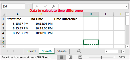
Step 2: We will use simple formula (end time – start time) to calculate the time difference, i.e., $B2-$A2

Step 3: Hit the Enter key and get the calculated result for the first row data.

The resultant time difference data is in h:mm:ss format, i.e., 02:02:29, which means 2 hours, 2 minutes, and 29 seconds.
Step 4: Drag the same formula in the below cells to calculate the time difference for other row’s data.

Step 5: Now, select one resultant cell (for now C2 cell) and press the Ctrl+1 to open the Format Cells dialogue box.

Step 6: On this dialogue box, move to the Custom tab in the left sidebar and select h:mm format then click OK.

Step 7: See that the time difference is changed to h:mm format in the C3 cell. Now, select another cell (C1) to change the format to h format.
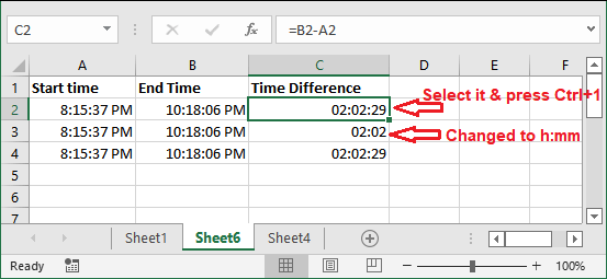
Step 8: Again, move to the Custom tab and type the h inside the Type field, then click OK. This time you have to manually enter the format, as h format is not available in the list.

Step 9: See that the time difference of C1 cell has changed to hours formats. See all time differences in different time formats.

Sometimes, you see that the time elapsed as hash marks (#####). This can be because of two reasons. One is your cell is not wide enough to store the result or another can be that your resultant time difference is a negative value. If you ever get the hash mark (#####) because of a negative time value, you can display these values.
We have described the way to display the negative value in this chapter below.
Example 2: Calculate and set the time difference using TEXT function
In the above method, you had manually set the custom time formats for different date differences. We will now use the TEXT format using which we will set the time format while calculating time differences. So, you do not need to set the date format manually.
We will calculate the time difference as well as assign the specific time format for each time difference. You will find this technique simpler than the above method.
The difference formula could be end time – start time, i.e., B2-A2. Its calculated result will be a string value.
TEXT formula with time format
Following are the codes for applying the custom formatting:
| Time Difference | Explanation |
|---|---|
| =TEXT(B2-A2, “h”) | Subtract a time from another and format the result in hours, e.g., |
| =TEXT(B2-A2, “h:mm”) | This elapses time in hours and minute, e.g., 3:10 |
| =TEXT(B2-A2, ” h:mm:ss “) | This elapses the time in hours, minutes, and seconds, e.g., 3:10:56 |
Step to subtract the time and get the result in different formats
Step 1: We have taken the time data (start time and end time). We will apply the TEXT function with all three date formats on each data individually so that you can understand all three formats described above.

Step 2: To calculate the time difference for the first row of data and get it in hours, write the formula in their adjacent cell (C2).
=TEXT(B2-A2, “h”)
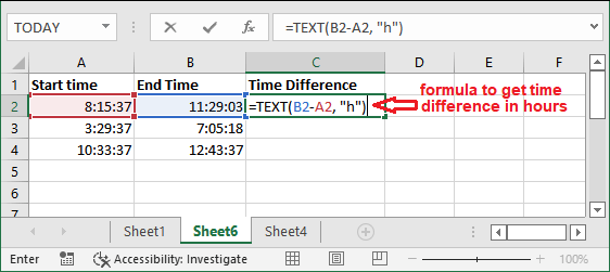
Step 3: Hit the Enter key and see the returned time in hours format.

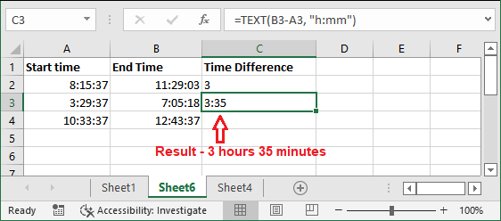
Step 4: Now, write the following formula in adjacent cell (C3) to get it in hours and minute format.
=TEXT(B2-A2, “h:mm”)

Step 5: Hit the Enter key and see the returned time in hours and minutes format.
Step 6: One more time, write the following formula in adjacent cell (C4) to get it in hours, minutes, and second format.
=TEXT(B4-A4, “h:mm:ss”)

Step 7: Hit the Enter key and see the returned time this time in hours, minutes, and second format.

In this way, you can specify the format for the calculated difference of time. So, you do not need to set the time format explicitly.
Example 3: Subtract time and get remaining time for task
Suppose that we have some tasks stored in an Excel sheet for which we have taken the assigned hours for each task and the working hours how much time work has been done. We will subtract time for the work done from total assigned hours for the task and find how much hour’s work remains.
See the Excel sheet data for this scenario.

The Excel user can use the following formula on data to get the time difference in a single unit.
Hours
To get the time difference in hours:
This is a very interesting formula whenever you need to find how many hours of work is remaining from total assigned hours. Using this formula, we can find how many hours of work have remained. We also have the formula for minutes and seconds.
Minutes
To get the time difference in minutes:
Seconds
To get the time difference in seconds:
Now, implement these formulas to the data that we had created above. But remember that after applying these formulas, you have to set the resultant column format to General format from Custom Formatting.
Steps to find remaining work hours
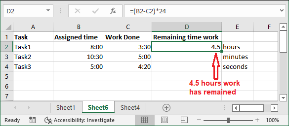
Step 1: First of all, calculate the remaining work hours for task1 by applying the below formula in D2 cell.
=(B2-C2)*24

Step 2: Now, press the Enter key to get the result. You will see that the resultant value is in h:mm format. So, change the format to General of the resultant value to get the result properly.

Step 3: Select the resultant cell and press the Ctrl+1 key.

Step 4: Move to the Custom tab in the right sidebar and select the General type for the selected data on this panel. Then, click OK.

Step 5: Now, you will find that the 4.5 hours of work have remained from the assigned hours.
In the same way, we will perform the same steps with task2 and task3 data to get the remaining time in minutes and seconds for the task to be done.
Steps to find remaining work minutes
This time we will calculate the remaining time of task2 in minutes rather than hours.
Step 1: Write the below formula in D3 cell to calculate the remaining work minutes for task2.
=(B3-C3)*1440

Step 2: Now, press the Enter key to get the result, but it shows 0:00 because it is formatted correctly for this formula. So, select the resultant cell and press the Ctrl+1 key.

Step 3: On this panel, move to the Custom tab in the right sidebar and select the General type for the selected data. Then, click OK.

Step 4: Now, you will find that the 330 minutes (5.5 hours) work has remained of task2 for the assigned hours to it.

Steps to find remaining work seconds
The last is to calculate the remaining time work in seconds instead of minutes or hours.
Step 1: Write the below formula in D3 cell to calculate the remaining work minutes for task2.
=(B4-C4)*86400

Step 2: Now, press the Enter key to get the result, but it again shows 0:00 because it is formatted correctly for this formula. So, select the resultant cell and press the Ctrl+1 key.

Step 3: On this panel, move to the Custom tab in the right sidebar and select the General type for the selected data. Then, click OK.
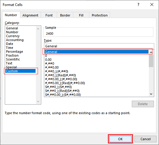
Step 4: Now, you will find that the 2400 seconds (40 minutes) work has remained of task3 for the assigned hours to it.

These all methods are for different scenarios and they also used different formulas in each. You have noticed that – we are subtracting the time in all these formulas to get the time difference result. Hence, you can use whatever method you need.
Example 4: Subtract AM/PM time
Till now, we had time in which AM or PM was not defined. But what if when the time meridian is also defined along with time? How does subtraction take place when you subtract time from another. So, let’s see an example for this too.
Step1: For this example, we have taken the following time dataset: start time and end time. This time, both time values are defined with AM and PM.

We have applied h:mm AM/PM on this data to define the date in this time meridian format.
Step 2: Now, we will apply the simple formula of subtraction formula to subtract a time from another. We are subtracting end time from start time.
=B2-A2

Step 3: Hit the Enter key and see the return result. But you see that the returned time difference is also in time meridian format. Because of that, the result looks like 4:35 AM (day time), but it is actually 4 hours 35 minutes.

So, we will change the format from h:mm AM/PM to h:mm format.
Step 4: Select the resultant cell and press the Ctrl+1 key to open the Format panel.

Step 5: On this panel, move to the Custom tab in the right sidebar and select the h:mm type for the selected data. Then, click OK.

Now, see the meridian has been removed from the time.
Step 7: After removing the meridian from time, select the resultant cell one more time and take the cursor to the bottom right corner that will enable a + sign. Drag this + symbol below till you want to calculate.
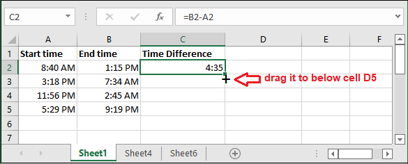
Step 8: See that all differences have been calculated for other cells, too, cell D3 and D4 having ##### as a result.

This is because the resultant time difference is a negative value and time cannot be negative. So, Excel returned hash code (######) as an error.
Display the negative time
In MS Excel, there is a way to display the negative time value (####) code. You have to change the Excel date system to 1904 date system. By setting the 1904 date system, -negative time will start displaying.
Follow the steps to change the date system to 1904:
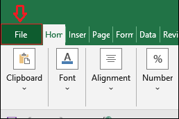
Step 1: Click on the File tab of this workbook containing ##### code error (negative time).
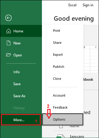
Step 2: Click More > Options on the Excel backscreen.
Step 3: On this panel, move to the Advanced tab on the left side of the panel.

Step 4: Now, scroll down to the “When calculating this workbooks” and mark the Use 1904 date system checkbox, then click OK.

Step 5: This time you see that the -negative time is also showing now after setting the 1904 date system.


