Closest Match
To find the closest match to a target value in a data column, use INDEX, MATCH, ABS and MIN in Excel. Use the VLOOKUP function in Excel to find an approximate match.
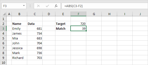
1. The ABS function in Excel returns the absolute value of a number.

Explanation: C3-F2 equals -39. The ABS function removes the minus sign (-) from a negative number, making it positive. The ABS function has no effect on 0 (zero) or positive numbers.
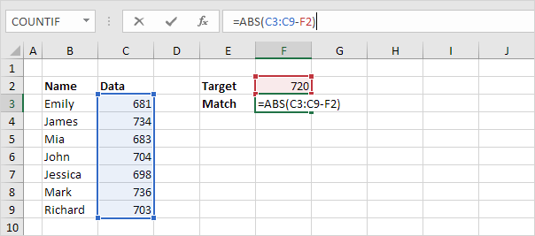
2. To calculate the differences between the target value and the values in the data column, replace C3 with C3:C9.

Explanation: the range (array constant) created by the ABS function is stored in Excel’s memory, not in a range. The array constant looks as follows:
{39;14;37;16;22;16;17}
3. To find the closest match, add the MIN function and finish by pressing CTRL + SHIFT + ENTER.

Note: the formula bar indicates that this is an array formula by enclosing it in curly braces {}. Do not type these yourself. The array constant is used as an argument for the MIN function, giving a result of 14.
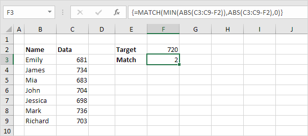
4. All we need is a function that finds the position of the value 14 in the array constant. MATCH function to the rescue! Finish by pressing CTRL + SHIFT + ENTER.

Explanation: 14 (first argument) found at position 2 in the array constant (second argument). In this example, we use the MATCH function to return an exact match so we set the third argument to 0.
5. Use the INDEX function (two arguments) to return a specific value in a one-dimensional range. In this example, the name at position 2 (second argument) in the range B3:B9 (first argument).

6. Finish by pressing CTRL + SHIFT + ENTER.

Next Chapter: Financial Functions


