Top Most Used Functions
Let’s check out the 10 most used Excel functions. Visit our section about functions for detailed explanations and more awesome functions.
Tip: download the Excel file and try to insert these functions.
1. COUNT
To count the number of cells that contain numbers, use the COUNT function in Excel.

Note: use COUNTA to count all cells that are not empty. COUNTA stands for count all.
2. SUM
To sum a range of cells, use the SUM function in Excel. The SUM function below sums all values in column A.


Note: you can also use the SUM function to sum an entire row. For example, =SUM(5:5) sums all values in the 5th row.
3. IF
The IF function checks whether a condition is met, and returns one value if true and another value if false.

Explanation: if the score is greater than or equal to 60, the IF function shown above returns Pass, else it returns Fail. To quickly copy this formula to the other cells, click on the lower right corner of cell C2 and drag it down to cell C6.
4. AVERAGE
To calculate the average of a group of numbers, use the AVERAGE function (no rocket science here). The formula below calculates the average of the top 3 numbers in the range A1:A6.

Explanation: the LARGE function returns the array constant {20,15,10}. This array constant is used as an argument for the AVERAGE function, giving a result of 15.
5. COUNTIF
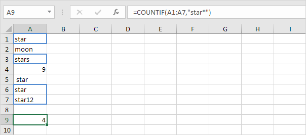
The COUNTIF function below counts the number of cells that contain exactly star + a series of zero or more characters.

Explanation: an asterisk (*) matches a series of zero or more characters. Visit our page about the COUNTIF function for more information and examples.
6. SUMIF
The SUMIF function below sums values in the range B1:B5 if the corresponding cells in the range A1:A5 contain exactly circle + 1 character.

Explanation: a question mark (?) matches exactly one character. Visit our page about the SUMIF function for more information and examples.
7. VLOOKUP
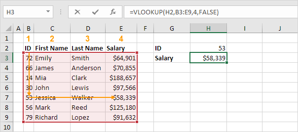
The VLOOKUP function below looks up the value 53 (first argument) in the leftmost column of the red table (second argument). The value 4 (third argument) tells the VLOOKUP function to return the value in the same row from the fourth column of the red table.

Note: visit our page about the VLOOKUP function to learn more about this powerful Excel function.
8. MIN
To find the minimum value, use the MIN function. It’s as simple as it sounds.

9. MAX
To find the maximum value, use the MAX function.

Note: visit our chapter about statistical functions to learn much more about Excel and Statistics.
10. SUMPRODUCT
To calculate the sum of the products of corresponding numbers in one or more ranges, use Excel’s powerful SUMPRODUCT function.

Explanation: the SUMPRODUCT function performs this calculation: (2 * 1000) + (4 * 250) + (4 * 100) + (2 * 50) = 3500.
Next Chapter: Ribbon


