
NOT Function in Excel
NOT Function
Th NOT function in Excel is an inbuilt function. The NOT function belongs to the category of Logical functions. We can use it as a worksheet function; the NOT function can be entered as part of a formula in a worksheet’s cell.
We can use it as an individual function or as a part of a formula and other excel functions in a cell. For example, with IF, AND & OR function. The NOT function is used to reverse a logical value. It returns the opposite value of a given logical value in the formula. If the value of the argument is TRUE, then it will return FALSE and vice versa.
Syntax
The syntax of the NOT function is:
Arguments or Parameters
logical_value: – An expression that either evaluates TRUE or FALSE. If we used with the expression of TRUE, then FALSE is returned. If used with the expression FALSE, then TRUE is returned.
Returns
- If the logical_value is TRUE, then the NOT Function will return
- If the logical_value is FALSE, then the NOT function will return
How to Use the NOT Function in Excel?
The NOT function in Excel is quite simple and straightforward to use. Let’s look at some examples of how to use the NOT function in Excel.
Example 1: In this example, the NOT function is used to perform a logical test on the given collection of data (Student score). We’ll check which value is larger than or equal to 60.
The table has two columns: the first column comprises student score & the second column is the logical test column, where the NOT function is performed.
Result: It will give us the opposite result or reverse value. If the value is larger than or equal to 60, the output will be FALSE; if the value is less than or equal to 60. Then the output will be TRUE.

After applying the formula, the result would be:

Example 2: Use NOT Function to Exclude Some Specific Values
In this example, we have a list of vegetables; we may want to exclude Brinjal, which we don’t like. So, if we use the NOT function, all Brinjal will return FALSE, whereas if we don’t, TRUE will be returned.
The formula we

Note:
1. If we wish to test many conditions in a single formula, we can use NOT with the AND or OR For example, if we need to exclude Brinjal and Carrot, the formula would be:

2. Also, if we wish to exclude brinjal from North, use NOT in conjunction with the Excel AND function.

Example 3: Use NOT Function to Deal with Blank Cells
It is another common usage of the NOT function; we can combine the NOT and ISBLANK functions in order to deal with certain blank cells while applying a formula, which is another typical use of the NOT function.
For example, we have a report with employee’s sales, and someone has completed the work excessively. They will receive a bonus if they have extra sales, that equals extra sales*10%. No incentive if their extra sales are blanks.
We may use this formula to combine the NOT and ISBLANK functions, which will give us the following result:

Example 4: NOT Function along with “IF” and “OR” Function
In this example, the color check is performed for the bike in the table below using the NOT Function, and the “IF” and “OR” function.
We need to sort out the color “BLUE” or “BLACK” from the given data set.
We will use the below formula:
This logical condition is applied on a Color column comprising any bike with the color “BLACK” or “BLUE”.
If the condition is true, then the output will be blank.
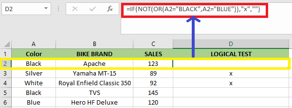
It the condition is not true, then the output will be “x”.

Example 5: NOT Function for an Empty Cell or Blank or “0”
The blank cell or empty cell or “0” are considered false, therefore the “NOT” function returns TRUE.
Here in the cell “C2”, the stored value is “0” suppose we use NOT function with logical arguments or value as “0” or “C2”, the result will be TRUE.

Example 6: NOT Function for Decimals
Suppose the value in the cell is a decimal value. Let’s assume we take the argument as decimals mean if we use the “NOT” function with a logical argument or values as “456.45” or “B2”. The result will be FALSE.

Example 7: NOT Function for Negative Number
If the value is a negative number in a cell. Suppose we use a negative number as the parameter; for example, if we use the “NOT” function with a logical argument or value as “-2” or “A2”, the result will be FALSE.

Example 8: When the Value or Reference is Boolean Input in NOT Function
If the value or reference is Boolean input (“TRUE” OR “FALSE”) in a cell. In this example, the cell A2, a FALSE value is stored so, if we use the “NOT” function with logical argument or value as “A2” or “FALSE”, the result will be TRUE. If the logical argument is “TRUE,” it will be vice versa means the NOT function returns the “TRUE” value as an output.

Example 9: Consider the following scenario: We have a head office in Paris and a number of regional offices. If the site is anything other than Paris, then we need to display the word “Yes,” and if it is Paris, we need to display the word “NO.”

The NOT function is nested in the logical test of the IF function given below in order to reverse the TRUE result.

The NOT Logical operator of <> can also be used to do this. Below is an example.

Example 10: When working with Excel’s information function, the NOT function is helpful. There are a set of Excel functions that check something and return TRUE if the check is successful and FALSE otherwise.
For example, the ISTEXT function will determine whether a cell contains text and return TRUE if it does or FALSE if it does not. The NOT function is useful if it is capable of reversing the result of these functions.
In the below example, we need to pay a salesman 15% of the amount they upsell. However, if they did not upsell anything, the word “None” will appear in the cell, resulting in a formula error.
We used the ISTEXT function to check the Text’s presence. If text is present, then it returns TRUE. Hence the NOT function returns FALSE, And the IF performs its calculation.

Example 11: Let’s say we do not want our soft toys to be Blue and Green. We have the below dataset:

We will use the formula =NOT(C2=”Blue Green”) to prevent the Blue Green combo.
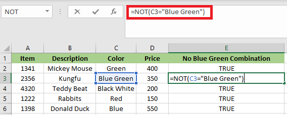
After applying the mentioned formula, we will get the output below:


