Slicers
Use slicers in Excel to quickly and easily filter pivot tables. Connect multiple slicers to multiple pivot tables to create awesome reports.
Below you can find a pivot table. Go back to Pivot Tables to learn how to create this pivot table.

To insert a slicer, execute the following steps.
1. Click any cell inside the pivot table.
2. On the Analyze tab, in the Filter group, click Insert Slicer.

3. Check Country and click OK.

4. Click United States to find out which products we export the most to the United States.

Conclusion: bananas are our main export product to the United States. The report filter (cell B1) changes to United States.
OK, that was pretty easy. Let’s insert a second slicer.
5. Click any cell inside the pivot table.
6. On the Analyze tab, in the Filter group, click Insert Slicer.

7. Check Product and click OK.

8. Select the slicer.
9. On the Options tab, in the Slicer Styles group, click a slicer style.

10. Use the second slicer. Click the Multi-Select button to select multiple products.

Note: instead of using the Multi-Select button, hold down CTRL to select multiple items.
To really impress your boss, execute the following steps.
11. Insert a second pivot table.
To connect both slicers to this pivot table, execute the following steps.
12. Select the first slicer.
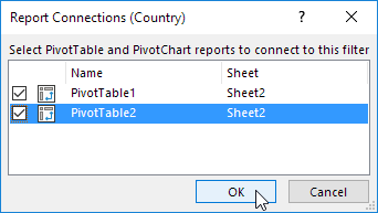
13. On the Options tab, in the Slicer group, click Report Connections.

14. Select the second pivot table and click OK.

15. Repeat steps 12-14 for the second slicer.
16. Use both slicers.

Conclusion: the total amount of apples exported to Canada equals $24,867 (6 orders) and the total amount of oranges exported to Canada equals $19,929 (3 orders).
17. Click the icon in the upper-right corner of a slicer to clear the filter.

Note: we didn’t export any beans or carrots to Canada. Try it yourself, download the Excel file and use slicers to create awesome reports.
Next Chapter: Tables


