What is Relative Reference in Excel

In Excel, Relative Reference is a kind of cell reference. Relative reference changes when the formula is copied to any other cell or any other worksheet. We used relative reference when calculations must be repeated.

In other words, a relative reference refers to the point of reference applied to a cell or a formula that returns a value which is relative to the cell location. There are mainly two types of cell references: Relative and Absolute. Relative and absolute references act differently when copied and filled to other cells. Relative references change whenever a formula is copied to another cell. But on the other hand, absolute references remain constant regardless of where they are copied. The row and column can both be kept constant with the use of absolute reference. A dollar sign ($) can be used in the formula to accomplish this. We have to put the dollar sign ($) before the row and column.

In Excel, a relative reference is the same as selecting a cell but not filling it with data. As a result, the cell value will not be fixed, and every time we copy or use that cell, its value will be modified along with the sheet’s reference. By default, all cell references are relative references. They change depending on the relative position of rows and columns when replicated across many cells. For example, the formula=A1+B1 will become =A2+B2 if we copy it from row 1 to row 2. When we need to repeat a calculation across numerous rows or columns, relative references are extremely useful.

How Relative References in Excel Change?

In relative references, every reference cell changes when we move up, down, left, or right. By default, each cell in Excel has a relative reference.

For example, if we give reference to cell B10 and move the cell in the below way:

• Upward- The reference change to B9.
• Downward- The reference change to B11.
• Leftward- The reference change to A10.
• Rightward- The reference change to C10.

How to Create and Copy a Formula Using Relative References

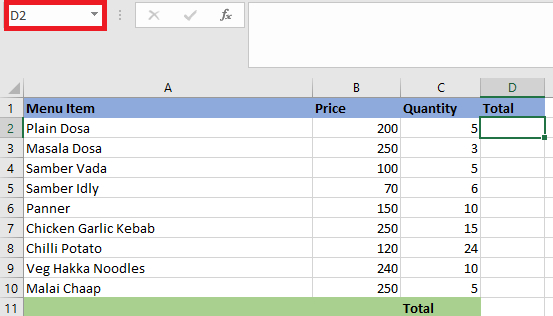
Let us understand the concept of relative reference with the help of the example. In the example below, we want to develop a formula that multiples the price of each item by the quantity. Instead of creating a separate formula for each row, we can build a single formula in cell D2 and copy it to the remaining rows. To ensures that the formula accurately calculates the sum for each item, we can use relative references.

We have to follow the following steps to create and copy a formula using relative references:

1. First, we have to select the cell where the formula will be entered. In this case, we’ll select the D2
   
2. Then, we have to type the formula to compute the desired value. In this example, we will type =B2*C2.
   
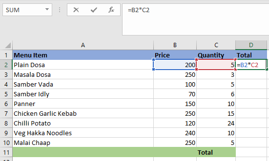
3. Then we have to press The formula will be calculated, and the result will appear in the cell.
4. Next, we have to locate the fill handle in the lower-right corner of the desired cell. In this example, we will locate the fill handle for cell
   
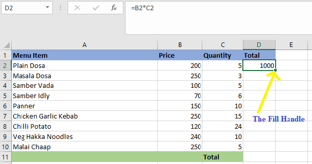
5. Fill the cells by clicking, holding, and dragging the fill handle over the cells. In this example, we will select cells D3:D10.
   
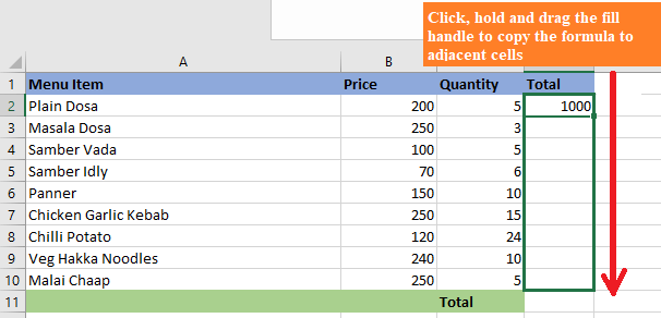
6. Next, we have to release the mouse. The formula will be copied to the selected cells with relative references, and values in each cell will be calculated.
   
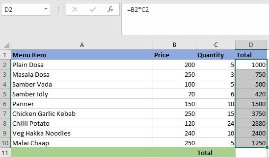
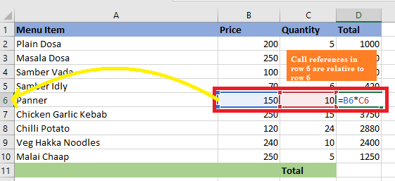
   • We can also double-click the filled cells to check their formulas for correctness. Depending on the row, the relative cell references must be different for each cell.
     

How to Use Relative References in Excel? (With Examples)

Let us explore more about relative references with the help of the following examples:

Example 1: With the help of an example, we can better comprehend the concept of relative cell references in Excel. A total of three numbers in cells A1, A2, and A3 is required. Let’s say we are looking for the sum in cell A4.

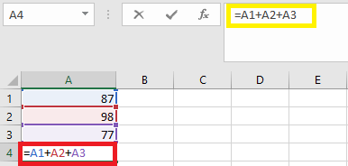
So, in cell A4, we have to apply the formula “=A1+A2+A2.”

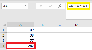
The sum of cells A1, A2, and A3 is equal to 262.

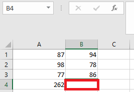
Now, with different values of cells B1, B2, and B3, we need a summation in cell B4.

There are two methods for calculating the total. We can use the Excel addition formula in cell B4 or copy and paste the formula form cell A4 to cell B4.

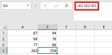
The answer is not 262 when copying cell A4 and putting it into cell B4. This is because cell A4, which is copied, has a formula rather than a value.

Cell A4’s output is depending on cells A1, A2, and A3. After copying cell A4, moving one cell to the right after copying cell A1, becomes B1, A2 becomes B2 and A3 becomes B3. As a result, cell B4 sums the values of cells B1, B2, and B3.

Example 2: Let’s look at another Excel example of relative references. The equation Units Sold*Unit Price=Sales Revenue will be used to determine the sales revenue.

In order to calculate the sales revenue, we multiple the number of units sold by the unit price.

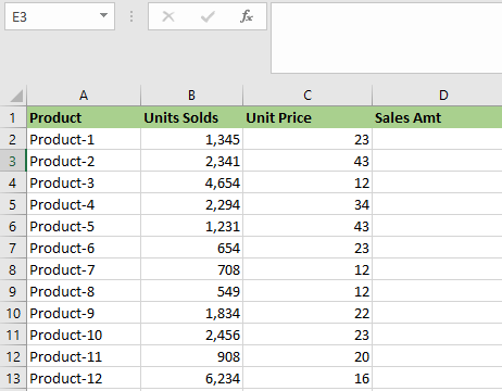
The sales income for product-1 is calculated using the formula B2*C2. It would be cumbersome to apply this formula to all items. As a result, we copy and paste the formula into the remaining cells.

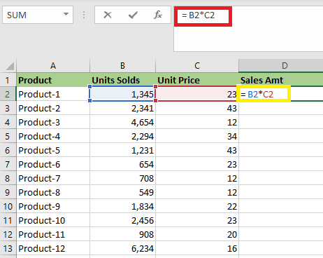
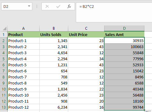
The formula reference changes from B2*C2 to B3*C3 as we copy the formula from cell D2 to cell D3. Press Ctrl+D or copy and paste cell D2 into the selected cells to determine the sales revenue for all products.

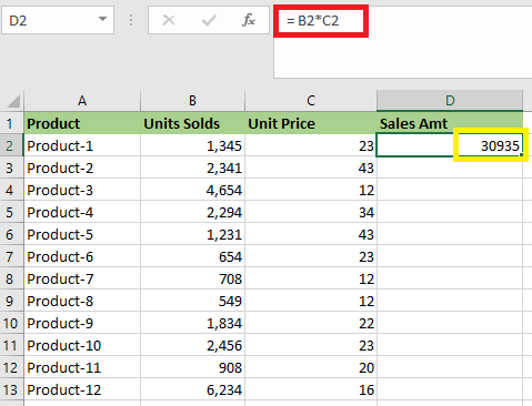
Writing the formula for the product would have taken a minute, but copying or dragging the fill handle merely takes a few seconds. So, we will drag the fill handle into the remaining cell to determine the sales revenues for all the remaining products.

Example 3: Let’s discuss more about relative references by using this example. In this example, we have to find out the student’s Body Mass Index. This is to determine the students’ health risks and whether they are in a healthy weight range. The weight (kg) and height (m) data of few students are already available.

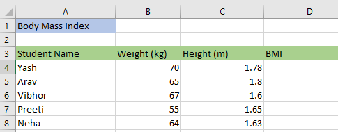
In order to calculate the BMI, we have to use the formula is =kgm^2.

In Yash’s case, it will be = 70/(1.78*1,78), or in Excel expression, it would be =B4/(C4*C4)

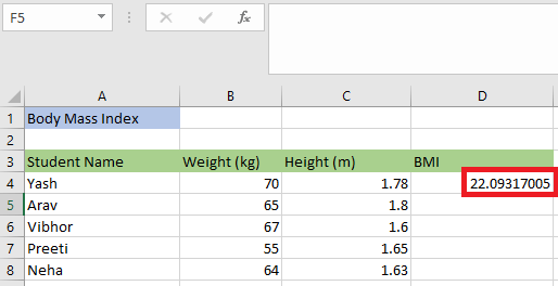
The return value is 22.09317.

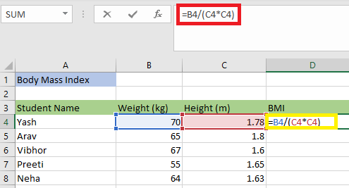
In order to calculate the remaining one, we have to simply copy and paste the formula in cell E4 and apply it to the rest of the cells (D5, D6, D7, D8).

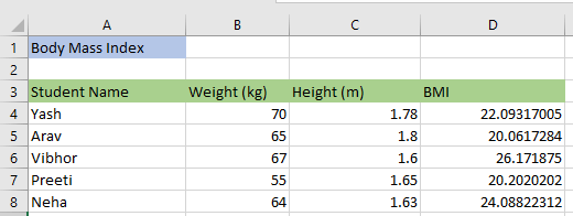
The data sets in this example are all variable. Each student is different in weight and height. The only thing they have in common is the computation of their BMI, which needs us to use the identical formula for each student.