Calculating skewness in Excel

Example 1 Calculate Skewness using SKEW function
Excel provides SKEW function. Syntax is:
=SKEW(number1, [number2], …)
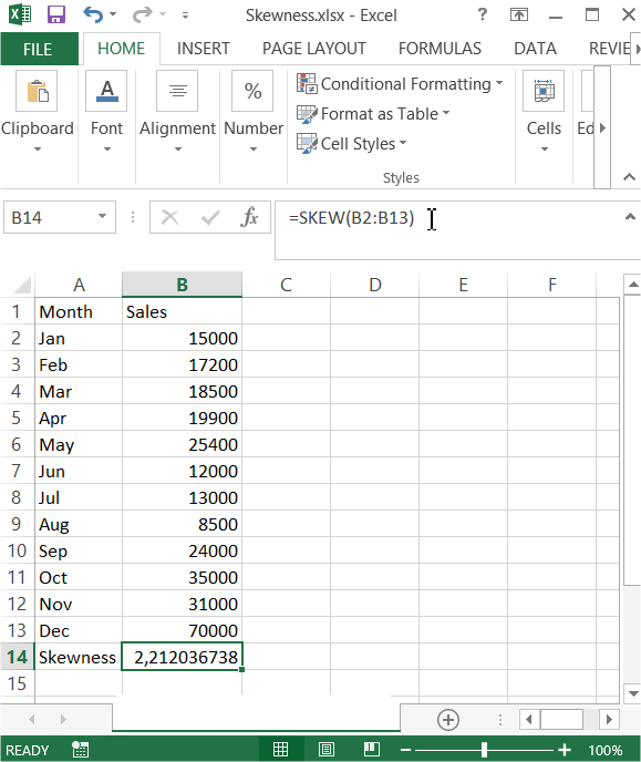
In this example formula is: =SKEW(B2:B13)

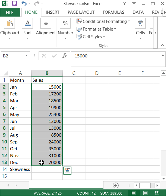
Skewness here is strongly above 0 (skewness > 0) what means that it is a right-sided asymmetry. The conclusion is that for many of months, sales was significantly lower than the average sales.
Example 2 Calculate Skewness using Data Analysis ToolPak Add-In
First you need to make sure your Data Analysis Toolpak Add-In is installed. Here is the lesson how to install Data Analysis Toolpak Add-In.
Go to Ribbon to the Data tab. Click the Data Analysis button.

New window appears. Choose Descriptive Statistics and click OK.

Enter the proper parameters:
- Input Range – range of your data ($B$1:$B$13 in my example)
- Labels in first row – there are labels in my data table
- Output Range – choose where you want to get your skewness calculated (I chose the same Sheet $E$1:$F$15)
- Summary statistics – make sure it is checked

And this is how to see my Statistics summary. Skewness is calculated in row 10. The result is the same as in the Example 1 where we checked how to calculate Skewness using SKEW Excel function.

Excel really helps you with statistics. Hopefully now you can see that.


