How Many Rows and Columns in Excel 2007?
The number of rows, columns, cells, and sheets supported by a spreadsheet depends on the software used and the spreadsheet’s data.
- Rowsrun horizontally and are identified by numbers (1, 2, 3, 4….).
- Columnsrun vertically and are identified by letters (A, B, C, D….).
This is the common question you can expect in an interview that requires excel skills. Many of us have not even looked at the last row or last column in a worksheet because we have never faced the situation we needed to go to the last row or last column.
If you have been using Excel 2003 for several years, you will probably be aware of increasing numbers of people or organizations using the latest Excel versions such as 2007, 2010, 2013, or Excel 2016. You may even have been sent Excel workbooks that you can’t open with your own version of Excel.
The main changes occurred between Excel 2003 and Excel 2007. Therefore, this page discusses some of the major changes between these two versions of Excel.
| Version | Number of Rows and Columns |
|---|---|
| Excel 2003 | 65,536 rows and 256 columns |
| Excel 2007 and later versions | 1,048,576 rows and 16,384 columns |
One of the main developments in Excel 2007 and later versions of Excel is that Excel now allows more columns and rows. Therefore, Excel’s recent versions’ ability to handle 1,048,576 rows and 16,384 columns of data is a great advantage for users.
Determining the Rows and Column Number
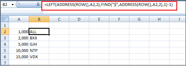
To know the number of rows is easy, but it’s much more complicated with the column header. How you can quickly determine what the header for column 2000 is by using the following formula.
Step 1: Enter a number of the column into a cell for which you want to find the column header.

The column header for the 1000th column is ALL, the column header for the 2000th column is BXX, and so on.
Here are some ways or shortcuts to get several rows and columns of a worksheet in Excel, such as:
1. How to get to the last row of a worksheet?
Press and hold down the Ctrl and press the down arrow key on the keyboard. You are taken to the bottom row.
In the latest versions of Excel, there are 1,048,576 rows. In older versions of Excel (2003 and prior), there were 65,536 rows.
2. How to get to the last column of a worksheet?
Press and hold down the Ctrl and press the right arrow key on the keyboard. You are taken to the right-most column.
In the latest versions of Excel, this is column XFD, which is 16,384 columns. In older versions of Excel (2003 and prior), the last column was IV which is 256 columns.
3. How many sheets are there in an Excel workbook?
By default, there are three sheets in a new workbook in all Excel versions, though users can create as many as their computer memory allows. These three worksheets are named Sheet1, Sheet2, and Sheet3. But it also has an option to add more sheets to the workbook.
4. How many characters can fit into a single cell?
The total number of characters a cell can contain is 32,767.
5. How are rows and columns labeled?
In all spreadsheet programs, including Microsoft Excel, rows are labeled using numbers (e.g., 1 to 1,048,576). All columns are labeled with letters A through Z, then AA through ZZ, etc.
For example, after the letter Z, the next column is AA, AB, AC, …, AZ, and then incrementing to BA, BB, BC, etc.
To identify a cell, give both the column and the row. For example, the first cell is always located in column A, on row 1, so the cell is labeled A1.
Main Developments in Excel 2007
Here are some major developments in Excel 2007 and the latest versions of Excel, such as:
1. Conditional Formatting
Another major improvement in Excel 2007 is Conditional formatting. Many users of Excel 2003 required the ability to apply more than 3 conditional formats, but this was not possible in Excel 2003. However, in Excel 2007 (and later versions of Excel), you can specify as many conditions as you want, each with a different format. In Excel 2007 and later versions, Conditional formatting can work for cells that satisfy more than one condition.
For example, if you specify cells with values ≤ 10 to have bold text and cells with values ≥ 10 to have red text, you will find that text in cells containing values exactly equal to 10 will be formatted as bold and red.

Also, Excel 2007 offers additional types of conditional formatting. You can illustrate data with charts and lots of colors. They will make attractive and easy-to-understand spreadsheets with Excel’s new Data Bars, Color Scales & Icon Sets.
These features apply color or symbols to a range of cells, depending upon each cell’s value with the rest of the selected range cells.
The above example shows conditional formatting Data Bars, Color Scales & Icon Sets applied to 3 columns, each containing 1 to 10.
As a final bonus, Excel 2007 introduced the ability to use conditional formatting with pivot tables.
1. Filtering and Sorting by Color
In Excel 2003, Filtering and Sorting could be performed by cell values only. However, in recent versions of Excel, you can filter and sort by color. This can be either the font color or the cell background color.
2. Function Nesting Limitations
Another useful improvement in Excel 2007 is the level of nesting that can be performed. Excel 2003 only allows 7 levels of nesting of functions, while Excel 2007 allows up to 64 levels of nesting functions. Surely, even the most dedicated Excel user cannot need more nesting levels than 64 levels.
3. Resizable Formula Bar
In Excel 2003, if a cell contained a long formula or text string, the formula bar’s view would block some of your spreadsheet, which could be inconvenient when the cell was selected.
However, Microsoft addressed this problem in Excel 2007 by introducing a resizable formula bar, which extends in line with your cell contents.
4. New Functions
Excel 2007 contains several new built-in functions to help you to make your spreadsheet slicker and more efficient. These include the IFERROR Function, the SUMIFS function, and the new statistical AVERAGEIF, AVERAGEIFS, and COUNTIFS functions.
Later versions of Excel have been added further to the list of the built-in functions.
5. Increased Memory and Faster Calculations
Suppose your work in Excel 2003 has been slowed down by slow calculations when applying functions to large datasets.
In that case, you may benefit from the increased memory management that is available in more recent versions of Excel. This was introduced in Excel 2007 when memory management was increased from 1 gigabyte to 2 gigabytes.
6. New User Interface
In Excel 2007, the main user interface was restructured into a results-oriented interface.
Suppose you have been using Excel 2003 for several years and know exactly where to find the tools and functionality you regularly use.
You will almost certainly experience some frustration, to begin with, when you upgrade to a more recent Excel version and have to get used to the new ribbon interface.
Restrict Users Action to Minimal Rows and Columns
Generally, we don’t use all the rows and columns, so we may want to restrict the user’s action to minimal rows and columns.
For example, assume we need to show only 5 rows and 10 columns, so we show minimal rows and columns by hiding other rows. First, we will hide rows, and then we will hide columns in the following steps.
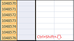
Step 1: Select other rows except for the first 5 rows. To select quickly, first select the 6th row and press the shortcut key “Ctrl + Shift + Down Arrow”. It will select all the remaining rows.

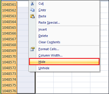
Step 2: Right-click on the row header and choose Hide, or you can press the shortcut key “Ctrl + 9,” and it will hide all the selected rows.

Step 3: Now, users can access only 5 rows, but all the 16k + columns, similar select all the columns except the first 10 columns.
Step 4: Now right-click on the column header and choose Hide or press the shortcut key “Ctrl + 0” to hide all the selected columns.

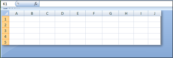
As you can see above, they can access only 5 rows and 10 columns.


