INDIRECT() function in Excel
INDIRECT() is an Excel in-built function. This function helps the users when they want to assemble the text value that can be used as a valid cell reference. The text passed inside this function is converted to a cell reference. Then if that converted reference cell contains any value, that value returns to the user back as a result.
For example, =INDIRECT(“B5”) It will refer to the B5 cell.
The main purpose of using this function is to create cell references from the text in an Excel worksheet. The INDIRECT() function creates the dynamic cell reference. As a resultant value, it returns the reference specified by a text string. It is a very interesting function.
Use of INDIRECT() function in Excel
The INDIRECT() function functionality is not limited; it helps a lot to achieve different results by creating dynamic cell reference. One of the greatest advantages of this formula is that – it does not change reference even when a new row or column is inserted/deleted.
Note: INDIRECT() function creates the dynamic cell reference.
An INDIRECT() function is useful for referencing a cell using text. It does not perform any arithmetic or logical calculation on Excel data. You can use it inside any other function and achieve the result. Due to dynamic cell reference functionality, we can change the cell reference within a formula without changing the formula itself.
Syntax
As simple as its definition, INDIRECT() function syntax is also very simple –
Here,
- Ref_text is the reference text string, and
- a1 is a logical value, TRUE or FALSE.
Second parameter ([a1]) is an optional parameter. When it is not passed, the INDIRECT() function considers it as TRUE.
- The type of reference in ref_text is specified by the a1.
- If the a1 is TRUE or not provided in INDIRECT() function, ref_text is interpreted as A1 Style cell reference.
- If A1 is FALSE, ref_text will be treated as R1C1 style cell reference.
Return Value
The INDIRECT() function returns the reference of the cell passed as a text in double-quotes inside the INDIRECT() function.
Cell reference Style
There are two types of cell references, i.e.,
- A1 Style cell reference
- R1C1 Style cell reference
Both are just opposite to each other. You should know about these style cell references to understand the INDIRECT() function because ref_text parameter values depend on it.
1. A1 Style cell reference
A1 Style cell reference is a usual reference type in Excel. It is a preferable style cell reference to use. In A1 style cell reference, a column is followed by a row number. For example, F3. Here, F is column number and 3 is row number.
2. R1C1 Style cell reference
R1C1 Style cell reference is just opposite to A1 Style cell reference. Unlike A1 reference, a row is followed by a column number.
Note: In this style, you must have to provide in second parameter.
As the name implies of R1C1, R refers to row and C refers to column. For example, R2C4 will refer to second row fourth column, i.e., D2 cell. If there is no number after a letter (e.g., R3C), it means we are referring to the same row and same column.
Examples of INDIRECT() function
There are several basic and advanced level examples of INDIRECT() function. Firstly, we will show you both A1 and B1C1 style cell reference basic examples to explain how they work on Excel worksheets.
Example 1: A1 Style cell reference
1. We have the following data stored in an Excel worksheet. Here, we will use the INDIRECT() function to create a cell reference in A1 style cell reference.

2. Now, write an INDIRECT() formula with a text parameter that will reference to a cell. For example,
=INDIRECT(“C5”)
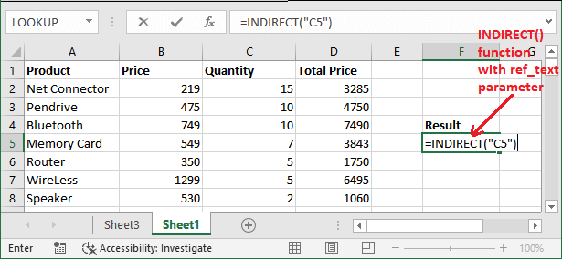
It will reference the C5 cell of this worksheet.
3. Hit the Enter key and get the resultant value stored in C5 cell.
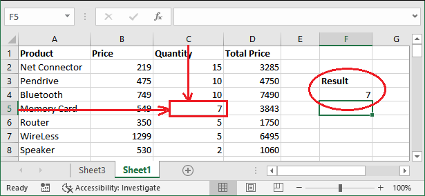
It returned the value 7 stored in C5 cell as INDIRECT() function converted the C5 text into the C5 cell reference.
Note: If the converted cell reference does not contain any value, the INDIRECT() function returns 0.
4. See that we have passed the E5 text string inside the INDIRECT() function, which is a reference of the E5 cell. E5 is an empty cell.
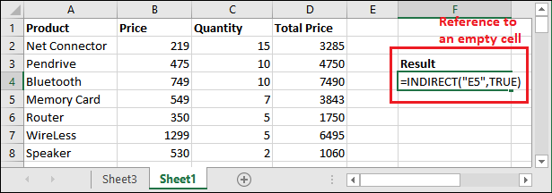
5. Get the result by pressing the Enter key and see it will return 0 as E5 cell does not contain any value. It is an empty cell.

Example 2: B1C1 Style cell reference
1. We have the same data as above stored in an Excel worksheet. Here, we will use the INDIRECT() function to create a cell reference in R1C1 style cell reference.
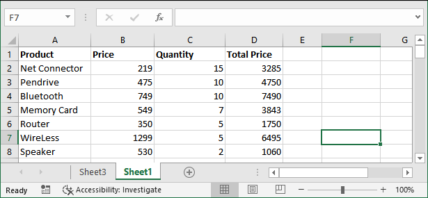
2. Write the following INDIRECT() formula with text parameter in R1C1 and FALSE as the second parameter value.
=INDIRECT(“R5C4”, FALSE)
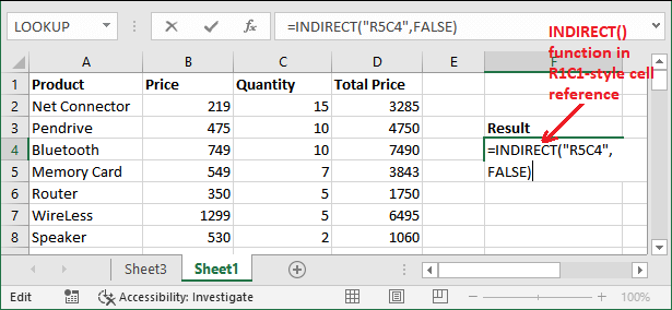
It is indicating to fifth row and fourth column. Thus, it will reference to the D5 cell of this worksheet.
3. Hit the Enter key to get the resultant value stored in D5 cell and see the value returned from it.
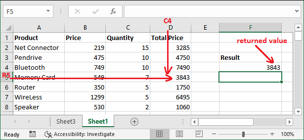
The INDIRECT() function had returned 3843 as the cell reference was D5. D5 cell is containing the total price of memory cards, i.e., 3843.
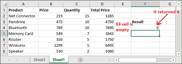
Note: Similar to A1-style cell reference, if a cell does not contain any value, INDIRECT() function will return 0 also in R1C1-style cell reference.
4. See that we have passed the R3C5 text string to the INDIRECT() function. It is a reference of E3 cell that does not contain any value.
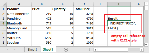
5. Get the result by pressing the Enter key and see it will return 0 as E3 cell does not contain any value. It is an empty cell.
These were the most basic and simple usage of the INDIRECT() function using both A1-style and R1C1-style cell reference.
INDIRECT() function with ROW()
Excel allows the users to use INDIRECT() function inside other functions and other functions nested inside the INDIRECT() function. They both together help to achieve special results and work dynamically.
Let’s understand through an example –
Step 1: We will fetch the cell data by creating the dynamic cell reference with INDIRECT() and ROW() functions.
Use the formula in this way:
=INDIRECT(“B” & ROW())
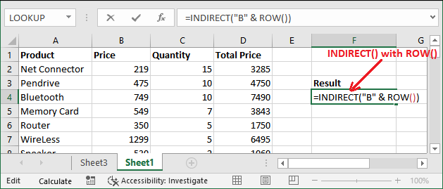
Firstly, the ROW() function will fetch the row number where your control is in Excel sheet that will later concatenate with the text string passed inside INDIRECT() function to convert in cell reference.
Step 2: Get the dynamic result for this formula. See that it has the value 749, which is stored in the B4 cell.
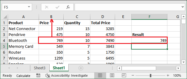
Here, ROW() function has returned row number 4 that concatenated with column B and returned the value stored in B4 cell by converting it to cell reference.
Advance usage of INDIRECT() function
INDIRECT() function is not only used for converting the simple cell reference. Additionally, it offers advanced functionality by allowing the use of it inside another function.
We can use this function with other Excel functions or nested inside it. For example, for calculating the sum of numbers by creating dynamic cell reference. Now, we will show you something different that how INDIRECT() function is used inside another to achieve the result.
Example 1: Sum of dynamic cell
Step 1: We have the following data, which is also used in the above examples. We will calculate the sum of cells by creating a dynamic cell reference.

Step 2: Write the following formula to get the dynamic sum of the total quantity of product. Quantity of each product is stored in column C.
=SUM(INDIRECT(“C2:C8”))
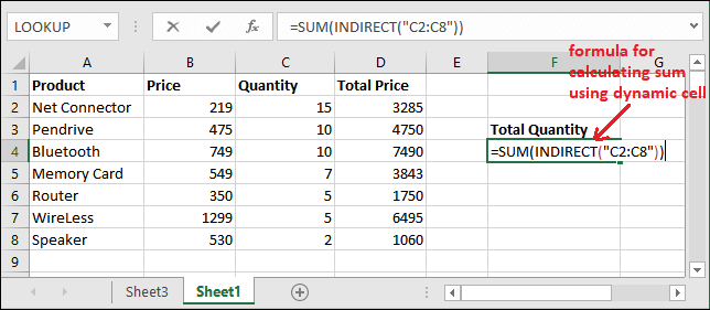
Step 3: Now, get the sum of the cells whose reference is generated by the INDIRECT() function. See that the total number of products is 54 calculated by this formula.
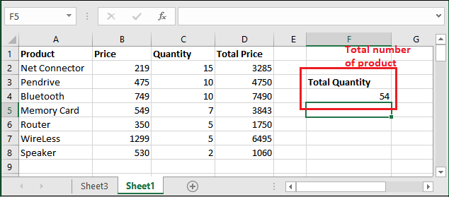
Similarly, we can use this formula to calculate the average of column data by replacing the SUM() with AVERAGE().
Example 1: AVERAGE of dynamic cell
Now, we will calculate the average of total price by creating the dynamic cell reference using the INDIRECT() function. The total price of each product is stored in column D.
Step 1: Write the following formula to get the average of the total price of the product.
=AVERAGE(INDIRECT(“D2:D8”))
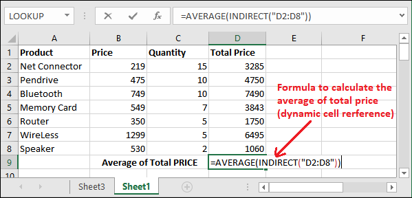
Step 2: Now, get the average of total price whose cell reference is generated by the INDIRECT() function. See that average of product total price is 4096.142857 calculated by this formula.
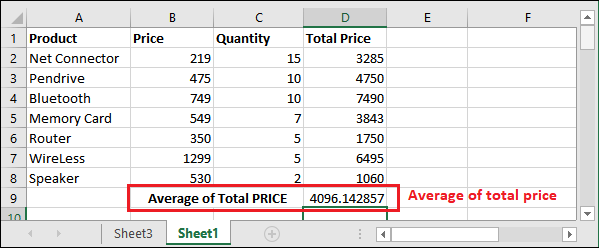
See how INDIRECT() function works with other functions. But now, you are thinking how this INDIRECT() function will help the users. INDIRECT() function locks the cell reference.
Look for the next example, “lock the cell reference using INDIRECT() function”.
Lock the cell reference using INDIRECT() function
Generally, we add or delete the rows and columns in Excel worksheets. It causes – the cell references that we used to manipulate the data, change automatically. The INDIRECT() function helps you to prevent changing the cell reference.
Here, we have a sum of the total quantity of all products. One is calculating simply with SUM() function and another average is calculated using SUM() with INDIRECT() function, i.e., (SUM(INDIRECT()).
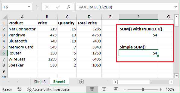
Now, if we insert a new column before the Price column for which we have calculated the average. See how it will affect the results of both formulas.
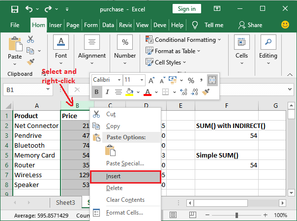
Here, you can see that a new blank column (column B) has been added to the worksheet, and the columns shifted to the right.
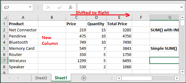
The result is that the Quantity column reference is changed from column C to column D, but the reference that we have created for column C did not change.
Effect on the calculated sum
Now see how it affects the calculated sum using both formulas.
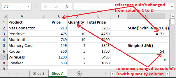
In this way, we lock the cell reference using the INDIRECT() function. The cell references do not change by adding or deleting the row/column that is set through the INDIRECT() function.
Here, you can clearly see that the –
SUM(INDIRECT(“C2:C8”)) – The cell reference created by the INDIRECT() function to calculate the sum is still same. Due to dynamic cell reference, it is still calculating the sum for column C, which is currently storing Price column details instead of Quantity.
SUM(“C2:C8”) – The cell reference in the simple SUM() formula has changed along with the column shifting. The cell reference is changed from column C to column D, and now it is still calculating the sum for column D. The column is currently storing Quantity column details.


